Why CRNN Works for OCR: A First-Principles Explanation for Developers New to AI

I recently built an OCR model that reads text from noisy images. The architecture was a CRNN - Convolutional Recurrent Neural Network - with CTC loss. It reached 98% accuracy.

But here’s what bothered me when I first learned about this architecture: nobody explained why these pieces fit together. Tutorials showed the code. Papers assumed background knowledge. I was left copying patterns I didn’t understand.

This post is the explanation I wish I’d had. We’ll build intuition from first principles: What problem are we solving? Why does each component exist? How do they connect?

No PhD required. Just curiosity.

The Problem: Reading Text from Images

Let’s be precise about what we’re trying to do:

Input: An image containing text (like “Hello” or “X7b9K”) Output: The text as a string

Sounds simple. It’s not. Here’s why:

1. Images are grids of pixels. A 128×32 image is 4,096 numbers (or 12,288 for RGB). The model sees no “characters” - just brightness values.

2. Text has variable length. “Hi” and “Hello World” are both valid outputs. The model must handle both.

3. Character positions are unknown. We know the image says “Hello”, but we don’t know exactly which pixels belong to which letter.

4. Characters depend on context. The letters “r” and “n” next to each other can look like “m”. Context matters.

Traditional software engineering would approach this with explicit rules: find edges, segment characters, match templates. This works for clean fonts. It fails catastrophically for noisy, distorted, or handwritten text.

Neural networks learn the rules from data. But which architecture learns these rules best?

Component 1: CNN for Feature Extraction

What it does: Turns raw pixels into meaningful features.

Why we need it: A pixel value of 127 means nothing by itself. But a pattern of pixels - an edge, a curve, a corner - means something. CNNs find these patterns.

How CNNs Work (The 30-Second Version)

A CNN slides small filters (like 3×3 grids of weights) across the image. Each filter detects a specific pattern:

Filter for vertical edge:    Filter for horizontal edge:
[-1  0  1]                   [-1 -1 -1]
[-1  0  1]                   [ 0  0  0]
[-1  0  1]                   [ 1  1  1]

Early layers detect simple patterns (edges, gradients). Later layers combine these into complex patterns (curves, shapes, parts of characters). The deepest layers recognize entire character fragments.

The Key Insight for OCR

After several CNN layers, our 128×32 image becomes something like a 32×8 “feature map” with 256 channels. What does this mean?

• Width reduced from 128 to 32: We’ve compressed horizontally, but preserved the left-to-right structure
• Height reduced from 32 to 8: Vertical information is compressed
• 256 channels: Each channel represents a different learned pattern

Think of it as: “For each of 32 horizontal positions, here are 256 features describing what patterns appear there.”

This is crucial. The CNN has converted our 2D image into something that’s almost a sequence - a series of feature vectors from left to right.

Image (128×32×3)
    ↓ CNN layers
Feature map (32×8×256)
    ↓ Collapse height
Sequence (32×256)

Component 2: Bidirectional LSTM for Sequence Modeling

What it does: Processes the feature sequence and adds context from both directions.

Why we need it: Characters aren’t isolated. What comes before and after matters.

The Context Problem

Consider these scenarios:

• “rn” vs “m” - Nearly identical visually. You need surrounding letters to disambiguate.
• “0” vs “O” - In “H2O”, it’s probably “O”. In “100”, it’s probably “0”.
• Partially obscured letters - The brain fills in gaps using context. So should our model.

A CNN processes each position independently. It doesn’t know what’s to the left or right. We need something that maintains memory across the sequence.

Enter the LSTM

LSTM (Long Short-Term Memory) is a type of recurrent neural network designed to remember information across long sequences. It processes one element at a time, maintaining a “hidden state” that summarizes what it’s seen.

For a sequence [x₁, x₂, x₃, x₄]:

Forward pass:  x₁ → x₂ → x₃ → x₄
               Each step sees what came BEFORE

Backward pass: x₁ ← x₂ ← x₃ ← x₄
               Each step sees what comes AFTER

Bidirectional means we run two LSTMs - one forward, one backward - and combine their outputs. Now every position has context from both directions.

What the LSTM Outputs

At each of our 32 positions, the LSTM outputs a vector. We pass this through a final linear layer to get probabilities over our character set.

If we have 62 characters (a-z, A-Z, 0-9) plus a special “blank” token (more on this later), we get:

Position 1: [P(a)=0.01, P(b)=0.02, ..., P(H)=0.89, ..., P(blank)=0.03]
Position 2: [P(a)=0.01, P(b)=0.02, ..., P(e)=0.85, ..., P(blank)=0.05]
...

Each position votes: “I think the character here is probably X.”

The Alignment Problem

Here’s where things get interesting - and where most tutorials lose people.

We have 32 positions outputting character probabilities. But “Hello” only has 5 characters. How do we map 32 outputs to 5 characters?

The naive approach: Define that positions 1-6 map to character 1, positions 7-12 map to character 2, etc. This requires knowing exactly where each character is in the image.

The problem: We don’t have character-level bounding boxes. Getting them would require expensive manual labeling. And characters aren’t evenly spaced - some are wide (W), some are narrow (i).

What we actually have:

• Input: Image of “Hello”
• Label: “Hello”

We don’t know which pixels correspond to which characters. We just know the whole image says “Hello”.

This is the alignment problem. And it’s why CTC exists.

Component 3: CTC Loss (The Clever Bit)

What it does: Lets us train without knowing character positions.

Why it’s brilliant: It considers all possible alignments between the model’s output and the target text.

The Blank Token

CTC introduces a special “blank” token (often written as - or ε). This token means “no character here” or “still on the previous character.”

With blanks, many output sequences can represent the same text:

Target: "Hi"

Valid alignments (all mean "Hi"):
- H-i--
- HH-ii
- -H-i-
- HHiii
- --Hi-

The rule: collapse repeated characters and remove blanks.

"HHH---iii" → "Hi"  (collapse HHH→H, remove ---, collapse iii→i)
"H-i-i-i"  → "Hii"  (H stays, blank removed, each i separated by blank = "Hii")

Wait, that last one is wrong! Let’s be precise:

"H-i-i-i" → collapse/remove → "H" + "i" + "i" + "i" = "Hiii"?

No. The rule is: collapse consecutive identical characters, then remove blanks.

"H-i-i-i": No consecutive identical characters. Remove blanks → "Hiii"

"HHH-iii": Consecutive H's collapse to H. Consecutive i's collapse to i. Remove blank → "Hi"

The blank lets us separate repeated characters:

"Hello" with double L:
"He-ll-o"  → "Hello" (no consecutive l's in output, they merge)
"He-l-l-o" → "Hello" (each l separated by blank, so we get two l's... wait)

Let me be even more precise:

Collapsing rule:
1. First, collapse consecutive identical NON-BLANK characters
2. Then, remove all blanks

"Hel-lo" → "Hel" + "-" + "lo" → collapse "ll"? No, they're not consecutive (blank between)
         → Remove blanks → "Hello" ✓

"Hello" (with no blanks) → collapse consecutive l's → "Helo" ✗

This is why blanks matter for repeated characters!

How CTC Training Works

During training, CTC computes the probability of all valid alignments that produce the target text, then maximizes this total probability.

For target “Hi” with output length 5:

P("Hi") = P("H-i--") + P("HH-i-") + P("-H-i-") + P("HHii-") + ...

The math involves dynamic programming (forward-backward algorithm), but the intuition is:

1. Sum probabilities of all paths that decode to the target
2. Backpropagate to increase this total probability
3. The model learns to make some valid alignment likely - it doesn’t matter which one

Why This Is Powerful

We never told the model where ‘H’ is or where ‘i’ is. We just said “this image says Hi” and let the model figure out the alignment.

This is why OCR models can be trained with just (image, text) pairs. No bounding boxes. No segmentation. Just the final answer.

How the Pieces Fit Together

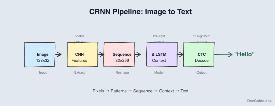
Let’s trace through the full pipeline:

Input: Image (128×32×3) of "Hello"

Step 1: CNN Feature Extraction
        Image → Feature map (32×8×256)
        "Find patterns at each horizontal position"

Step 2: Reshape for Sequence
        (32×8×256) → (32×2048) by flattening height×channels
        "Convert to a sequence of 32 feature vectors"

Step 3: Bidirectional LSTM
        (32×2048) → (32×512)
        "Add context from left and right neighbors"

Step 4: Linear + Softmax
        (32×512) → (32×63) where 63 = 62 characters + blank
        "Convert to character probabilities at each position"

Step 5: CTC Decode (inference) or CTC Loss (training)
        Training: Compute loss against target "Hello"
        Inference: Greedy decode or beam search → "Hello"

Each component solves a specific problem:

Component	Problem Solved
CNN	Raw pixels → meaningful features
Reshape	2D feature map → 1D sequence
BiLSTM	Independent positions → context-aware positions
CTC	Unknown alignment → trained without alignment labels

The Greedy Decoding Trick

During inference, how do we get text from probabilities?

Greedy decoding: At each position, take the most likely character. Then collapse and remove blanks.

Position outputs (most likely):
[H] [H] [-] [e] [l] [l] [-] [l] [o] [-] [-]

Collapse consecutive identical: H - e l - l o -
Remove blanks: H e l l o
Result: "Hello"

Beam search: Keep track of multiple hypotheses and pick the best complete sequence. More accurate but slower.

For most applications, greedy decoding works surprisingly well.

Why Not Just Use a Transformer?

Fair question. Transformers dominate NLP. Why use LSTMs for OCR?

1. Sequence length: OCR sequences are short (typically <50 positions). Transformers shine on long sequences where their O(n²) attention becomes worthwhile.

2. Inductive bias: LSTMs naturally process left-to-right, matching how we read. Transformers need to learn this from data.

3. Simplicity: CRNN has fewer hyperparameters and is easier to train on small datasets.

4. It works: 98% accuracy on our task. Sometimes boring is better.

That said, Vision Transformers (ViT) and attention-based OCR (like TrOCR) are increasingly popular. For large-scale production systems with massive training data, they often win. For a weekend project with 2,000 images? CRNN is hard to beat.

What I Wish I’d Known Earlier

1. Architecture follows problem structure.

OCR has inherent structure: 2D image → 1D text, spatial patterns → sequential characters, unknown alignment. CRNN mirrors this structure: CNN → RNN → CTC.

2. CTC is the key insight.

Everything else (CNN, LSTM) existed before. CTC is what made end-to-end OCR training practical. If you understand nothing else, understand CTC.

3. The feature sequence is the bridge.

The CNN’s output isn’t just “features” - it’s specifically arranged as a left-to-right sequence. This isn’t accidental. The architecture is designed so spatial position in the image maps to temporal position in the sequence.

4. Context matters more than you think.

Single-character recognition is easy. Reading words in noisy images requires understanding that “rn” is probably “rn” in “barn” but might be “m” in “summer”. The BiLSTM provides this.

Try It Yourself

The best way to understand is to implement. Here’s a minimal PyTorch CRNN:

import torch
import torch.nn as nn

class CRNN(nn.Module):
    def __init__(self, num_chars):
        super().__init__()

        # CNN: extract features
        self.cnn = nn.Sequential(
            nn.Conv2d(3, 64, 3, padding=1),
            nn.ReLU(),
            nn.MaxPool2d(2, 2),  # 128×32 → 64×16

            nn.Conv2d(64, 128, 3, padding=1),
            nn.ReLU(),
            nn.MaxPool2d(2, 2),  # 64×16 → 32×8

            nn.Conv2d(128, 256, 3, padding=1),
            nn.ReLU(),
        )

        # RNN: sequence modeling
        # Input: 256 channels × 8 height = 2048 features per position
        self.rnn = nn.LSTM(256 * 8, 256, num_layers=2,
                          bidirectional=True, batch_first=True)

        # Output: probability over characters (including blank)
        self.fc = nn.Linear(256 * 2, num_chars + 1)  # ×2 for bidirectional

    def forward(self, x):
        # x: (batch, 3, 32, 128)

        # CNN features: (batch, 256, 8, 32)
        conv = self.cnn(x)

        # Reshape: (batch, 32, 256×8) - width becomes sequence length
        batch, channels, height, width = conv.shape
        conv = conv.permute(0, 3, 1, 2)  # (batch, width, channels, height)
        conv = conv.reshape(batch, width, channels * height)

        # RNN: (batch, 32, 512)
        rnn_out, _ = self.rnn(conv)

        # Output: (batch, 32, num_chars+1)
        output = self.fc(rnn_out)

        return output

Train it with nn.CTCLoss. The PyTorch implementation handles all the dynamic programming.

The Fundamental Lesson

Architecture isn’t arbitrary. Good architectures encode assumptions about the problem:

• Images have spatial structure → Use convolutions
• Text is sequential → Use recurrence
• Alignment is unknown → Use CTC

When you encounter a new problem, ask: What structure does this problem have? What inductive biases would help? The answer often points to the architecture.

The CRNN wasn’t invented by trying random combinations. It was designed by people who understood both the problem (reading text from images) and the tools (CNNs for vision, RNNs for sequences, CTC for alignment). The architecture is a precise answer to a well-defined question.

That’s the lesson beyond OCR: understand your problem deeply, and the architecture often becomes obvious.

---

The model described here achieved 98% accuracy on 2,000 noisy images. The architecture is simple, the training is straightforward, and the results are good. Sometimes that’s all you need.