1 What is deep learning? (Summary)

1.1 AI, ML, DL

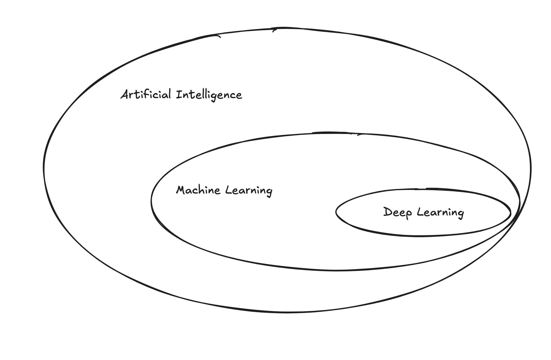
This is a summary of Chapter 1 of the book “Deep Learning” by François Chollet. The chapter covers the essential context around artificial intelligence, machine learning, and deep learning. Here are the key takeaways:

1.1.1 Artificial Intelligence (AI)

AI can be described as the effort to automate intellectual tasks that typically require human intelligence. It encompasses a wide range of techniques and approaches, including machine learning and deep learning.

1.1.2 Machine Learning

The usual way to make a computer do useful work is by programming it. However, this approach has limitations, especially when dealing with complex tasks. Machine learning offers an alternative approach. The machine looks at the input data and the corresponding output and learns the relationship between them. A machine learning system is ‘trained’ rather than explicitly programmed. It’s presented with many examples relevant to the task at hand and it learns a statistical structure in these examples that eventually allows the system to come up with rules for automating the task.

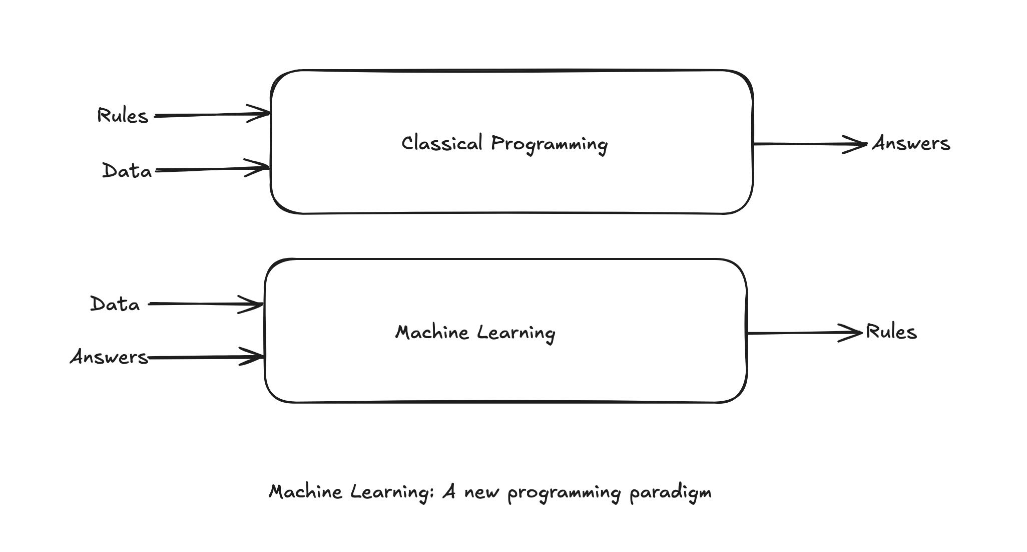
For example, if you wished to automate the task of distinguishing between images of cats and dogs, you would feed the machine many images of cats and dogs, and the machine would learn statistical rules that differentiate the two. Once trained, the machine can then classify new images as either cats or dogs.

Although, ML only started to flourish in 1990s, it has quickly become the most powerful and most successful subfield of AI, mainly because of the availability of faster hardware and larger datasets.

ML is related to mathematical statistics, but it differs from statistics in several different ways. Just like medicine is related to chemistry but cannot be reduced to chemistry, as medicine deals with its own systems with their own distinct properties.

Unlike statistics, ML tends to deal with very large, complex datasets(such as the dataset of million of images, each consisting of tends of thousands of pixels) for which classic statistical analysis, such as Bayesian analysis, would be impractical. As a result, ML, and especially deep learning, exhibits comparatively little mathematical theory, maybe too little, and is fundamentally an engineering discipline. Unlike theoretical physics, ML is a very hands-on field driven by empirical findings deeply reliant on advances in software and hardware.

1.1.3 Learning rules and representations from data

A machine learning model transforms its input data into meaningful outputs, a process that is learned from exposure to known examples of inputs and outputs. Therefore, the central problem in machine learning and deep learning is to meaningfully transform data: to learn useful representations of the input data at hand - representations that get us closer to the expected output.

What is representation? It’s a different way to look at data - to represent or encode data. For example, a color image may be encoded in the RGB format, or it may be encoded in the HSV format. The choice of representation has a significant impact on the performance of the model.

Machine learning models are all about finding appropriate representations for their input data - transformations of the data that make it more amenable tot the task at hand.

Let’s consider an example. Consider an x-axis, a y-axis and some points represented by their coordinates in the (x, y) system.

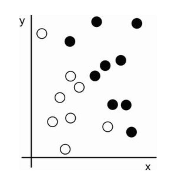
Let’s say we want to develop an algorithm that can take the coordinates (x, y) of a point and output whether that point is likely to be black or white. Here:

• The inputs are the coordinates of our points.
• The expected outputs are the color of the points.
• A way to measure whethere our algo is doing a good job could be, for instance, the percentage of points that are being correctly classified.

What we need here is a new representation of our data that cleanly separates the white points from the black points. One transformation we could use, among many other possibilities, would be a coordinate change.

In this new coordinate system, the coordinates of our points can be said to be a new representation of our data. With this representation, the black/white classification problem can be expressed as a asimple rule: “Black points are such that x > 0 and White points are such that x < 0”. The new representation combined with this simple rule, neatly solves the classification problem.

In this case we defined the coordinate change by hand: we used our human intelligence to come up with our own appropriate representation. But could you do the same if the task were to classify images of handwritten digits? Could you write down explicit, computer-executable image transformations that would illuminate the difference between a 6 and and 8, between a 1 and a 7, across all kinds of different handwriting?

Coding this intelligence by hand is hard work and the resulting rule-based system will be brittle, a nightmare to maintain.

If this process is so painful, could we automate it? What if we tried systematically searching for different sets of automatically generated representations of the data and rules based on them, identifying good ones by using as feedback the percentage of digits being correctly classified in some development data set? We would then be doing machine learning. Learning, in the context of machine learning, describes an automatic search process for data transformations that produce useful representations of some data, guided by some feedback signal - representations that are more conducive than solving the problem with simpler rules.

These transformations can be coordinate changes, or taking a histogram of pixels and counting loops, but the could also be linear projections, translations, nonlinear operations(such as select all points such that x>0), and so on.

ML algos aren’t usually creative in finding these transformations. They’re just searching through a predefined set of operations, called a hypothesis space, looking for the one transformation that minimizes the error in the training data. For instance, the space of all possible coordinate changes would be out hypothesis space in the 2D coordinations classification example.

So that is the essence of machine learning: searching for useful representations and rules over some input data, within a predefined space of possibilities, using guidance from a feedback signal. This simple idea allows for solving a remarkably broad range of intellectual tasks, from speech recognition to autonomous car driving.

1.1.4 The “deep” in deep learning

Deep learning is a specific subfield of machine learning: a new take on learning representations from data that puts an emphasis on learning successive layers of increasingly meaningful representations. The “deep” in “deep learning” isn’t a reference to any kind of deeper understanding achieved by the approach; rather, it stands for this idea of successive layers of representations. How many layers contribute to a model’s depth? This is called the depth of the model.

For our purposes, deep learning is a mathematical framework for learning representations from data.

You can think of a deep network as a multistage information-distillation process, where information goes through successive filters and comes out increasingly purified (i.e., useful for the task at hand).

It’s a simple idea, but as it turns out, very simple mechanism sufficiently scaled, can end up looking like magic.

1.1.5 Understanding how deep learning works

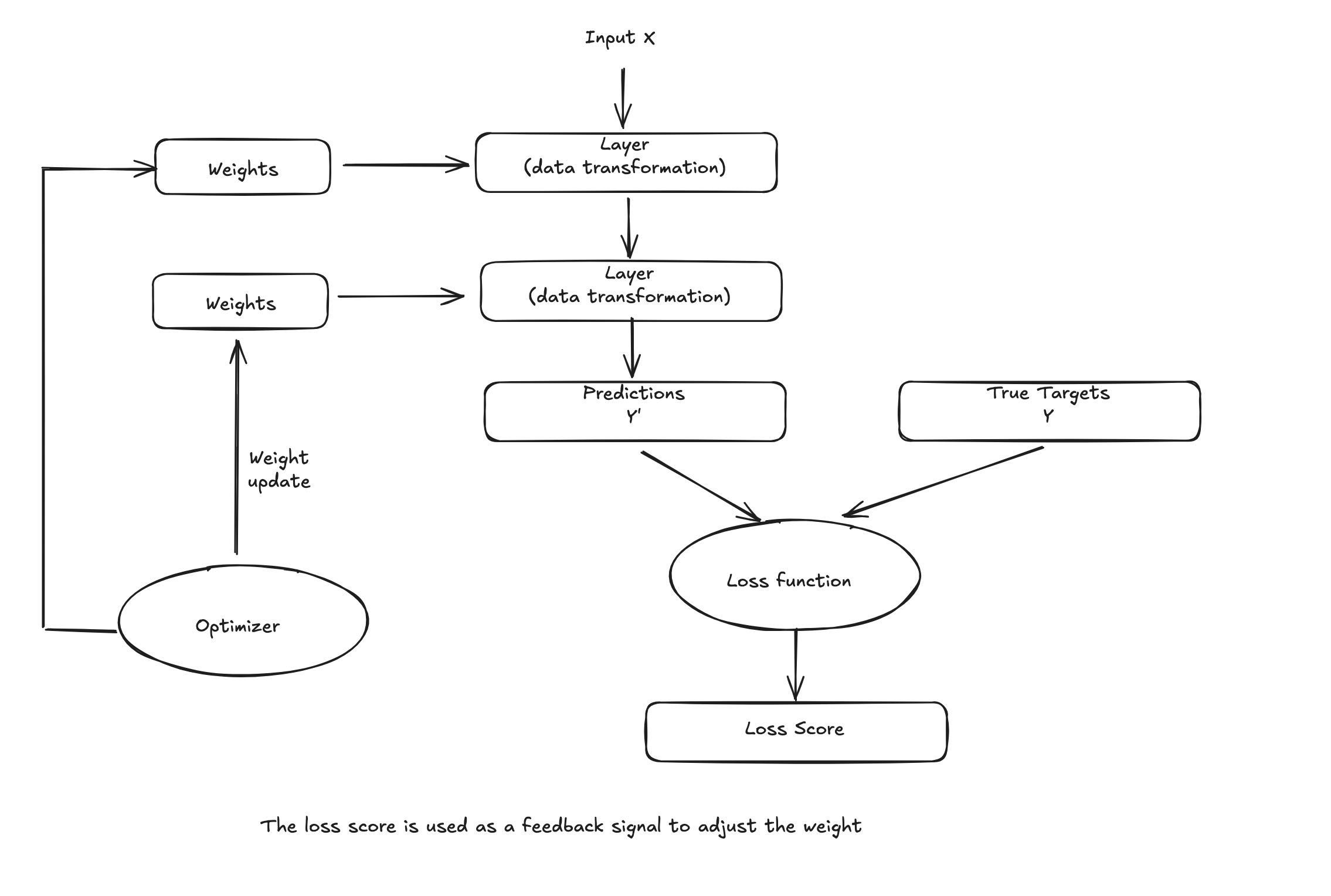
The specification of what a layer does to its input data is stored in the layer’s weights, which in essence are a bunch of numbers.

In this context, leraning means finding a set of values for the weights of all layers in a network, such that the network will correctly map example inputs to their associated targets. But here’s the thing, deep neural network can contain tens of millions of parameters. Finding the correct values for all of them may seem like a daunting task, especially given that modufying the value of one parameter will affect the behavior of all others!

The fundamental trick in deep learning is to use this score of feedback signal to adjus the values of the weights a little.

1.2 Before deep learning: A brief history of machine learning

It is safe to say that mosst of the ML algos used in the industry today aren’t deep learning algos. Deep learning isn’t always the right tool for the job- sometimes there isn’t enough data for deep learning to be applicable, and sometimes the problem is better solved by different algos.

We will go over classical ML algos and describe the historical context in which they were developed.

1.2.1 Probabilistic modeling

Probabilistic modeling is the application of the principles of statistics to data analysis. It is one of the earliest forms of ML, and is still widely used to this day. One of the best known algos in this category is the Naive Bayes classifier.

NB is a type of ML classifier based on applying Baye’s theorem while assuming that the feautres in the input data are all independent(a strong or naive assumption, which is where the name comes from).

Baye’s theorm and the foundation of statistics dates back to 18th century and these are all you need to start using Bayes classifiers.

A closely related model is logistic regression. which is sometimes considered to be a “Hello World” of modern ML. Don’t be misled by name, logreg is a classification algo, not a regression algo.

Much like Naive Bayes, logreg predates computing by a long time, yet its still used today, thanks to its simple and versatile nature. It’s often the first thing a data scientist will try on a dataset to get a feel for the classification at hand.

Early iteration of neural networks have been completely supplanted by the modern variants covered in these pages, but it is helpful to be aware of how deep learning originated.

The first successful application of neural nets came in 1989 from Bell Labs, when Yann LeCun combined the earlier ideas of convolutional neural network and backpropagation, and applied them to the problem of classifying handwritten digits. The resulting network, dubbed LeNet, was used by the US Postal Service to automate the reading of ZIP codes on mail envelopes.

1.2.3 Kernel methods

Kernel methods are a group of classification algos, the best of which is known as SVM(Support Vector Machine). The modern formulation of SVM was developed by Vladimir Vapnik and Corinna Cortes in the early 1990s at Bell Labs and published in 1995, although an older linear formulation was published by Vapnik and Alexey Chervonenkis in 1963.

SVM is a classification algorithm that works by finding “decision boundaries” separating two classes. SVMs proceed to find these boundaries in two steps:

1. The data is mapped to a new high-dimensional representation where the decision boundary acan be expressed as a hyperplane.( if the data is two dimensional, the hyperplane would be a straight line)
2. A good decision boundary( a separation plane) is computed by trying to maximize the distance between the hyperplane and the closest data points from each class, a step called maximizing the margin. This allows the boundary to generalize well to new samples outside the training dataset.

The technique of mapping data to a higher-dimensional representation where a classification problem becomes simpler may look good on paper, but in practice it’s often computationally intractable. That’s where the kernel trick comes in(the key idea that kernel methods are named after). Here’s the gist of it: to find good decision hyperplanes in the new representation space, you don’t have to explicitly compute the coordinates of your points in that space. You just need to compute the distance between pair of points in that space, which can be done efficiently using a kernel function. A kernel function is a computationally tractable function that maps any two points in your original space to the distance between these points in the target representation space, completely bypassing the explicitly computation of the new representation. Kernel functions are typically crafted by hand rather than learned from data - in case of SVM, only the separation hyperplane is learned from data.

At the time they were developed, SVM exhibited state-of-the-art performance on simple classification problems and were one of the few machine learning methods backed by extensive theory and amenable to serious mathematical analysis, making them well understood and easily interpretable.

But SVMs proved hard to scale to large datasets and didn’t provide good results for perceptual problems such as image classification. Because an SVM is a shallow method, applying an SVM to perceptual problems requires first extracting useful representations manually from data(a step called feature engineering), which is difficult and brittle.

1.2.4 Decision trees, random forests, and gradient boosting machines

Decision trees are flowchart-like structures that let you classify input data points or predict output values given by inputs. They are easy to visualize and interpret. Decision trees learned from data began to receive significant research interest in the 2000s and by 2010 they were often preferred to kernel methods.

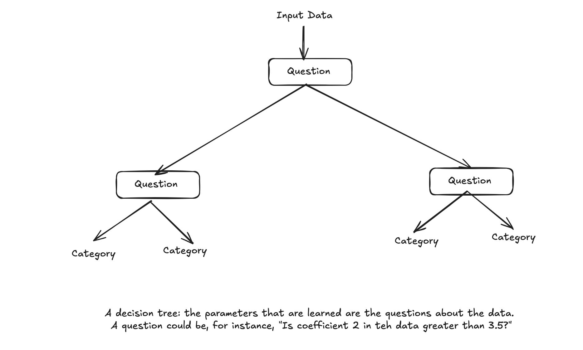
In particular the random forest algorithm introduced a robust, practical take on the decision tree learning that involves building a large number of specialized decision trees and then ensembling their outputs. Random forests are applicable to a wide range of problems - you could say that they’re almost always the second-best algorithm for any shallow ML problem.

A gradient boosting machine, much like random forests, is a ML technique based on ensembling weak prediction models, generally decision trees. It uses gradient boosting, a way to improve any ML model by iteratively training new models that specialize in addressing the weak points of the previous models. Applied to decision trees, the use of the gradient boosting technique results in models that strictly outperform random forests most of the time, while having similar properties. Gradient Boosting may be one of the best, if not the best, algorithm for dealing with nonperceptual data today. Alongside deep learning, it’s one of the most commonly used techniques in Kaggle comptetition.

1.2.5 Back to neural networks

Since 2012, deep convolutional neural networks(convnets) have become the goto algorithm for all computer vision tasks; more generally, they work on all perceptual tasks. Around 2015, the classification task of ImageNet was considered to be a solved problem. At the same time, deep learning has also found applications in many other types of problems, such as natural language processing. It has completely replaced SVMs and decision trees in wide range of applications. For instance, CERN switched to Keras-based deep neural networks due to their higher performance and ease of training on large datasets.

1.2.6 What makes deep learning different

The primary reason deep learning took off was that it offered better performance for many problems. But that’s not the only reason. Deep learning also makes problem-solving much easier because it completely automates what used to be the most crucial step in machine learning workflow: feature engineering.

Previous machine learning techniques - shallow learning - only involved transforming the input data into one or two successive representations spaces, usually via simple transformations such as high-dimensional non-linear projections(SVMs) or decision trees. But the refined representations required by complex problems generally can’t be attained by such techniques. As such, humans had to go to great lengths to make the initial input data more amenable to processing by these methods: they had to manually engineer good layers of representations for their data. This is called feature engineering.

Deep Learning on the other hand, completely automates this step of feature engineering. With deep learning, you learn all features in one pass rather than having to engineer them yourself. This has greatly simplified machine learning workflows, often replacing sophisticated multistage pipelines with a single, simple, end-to-end deep learning model.

You may ask, if the crux of the issue is to have multiple successive layers of representations, could shallow methods be applied repeateadly to emulate the effects of deep learning? In practice, successive applications of shallow-learning methods produce fast fast-diminishing returns, ** because the optimal first representation layer in a 3-layer model isn’t the optimal first layer in a 1-layer or 2-layer model.** What is transformative about deep learning is that it allows a model to learn oall layers of representation jointly, at the same time, rather than in succession(greedily, as it’s called). With joint feature learning, whenever the model adjusts one of its internal features, all other features that depend on it automatically adapt to the change, without requiring human intervention. Everything is supervised by a single feedback signal. Every change in the model serves the end goal. This is much more powerful than greedily stacking shallow models, because it allows for complex, abstract representations to be learned by breaking them down into long series of intermediate spaces(leayers); each space is only a simple transformation away from the previous one.

These are two essential characteristics of how deep learning learns from data:

1. Incremental, layer-by-layer way in which increasingly complex representations are developed, and
2. the fact that these intermediate incremental representations are learned jointly, each layer being updated to follow both the representational needs of the layer above and the needs of the layer below.

Together, these two properties have made deep learning vastly more successful than previous approaches to machine learning.

1.2.7 The modern machine learning landscape

In early 2019, Kaggle ran a survey asking teams that ended in the top 5 of any competition since 2017 which primary software tool they had used in the competition. It turns out that top teams tend to use:

1. Deep learning libraries most often via the Keras library.
2. Gradient Boosteed Trees, (most often via the LightGBM or XGBoost libraries)

From 2016 to 2020, the entire machine learning and data science industry has been dominated by these two approaches: deep learning and gradient boosted trees.

Specifically, gradient boosted trees is used for problems where structured data is available, while deep learning is used for perceptual problems such as image classification.

Users of gradient boosted trees tend to use Scikit-learn, Xgboost or LightGBM. Meanwhile, most practitioners of deep learning use Keras, often in combination with its present framework, TensorFlow.

These are the two techniques you should be most familiar with in order to be successful in applied machine learning today:

1. Deep learning, for perceptual problems
2. Gradient boosted trees, for shallow learning problems

1.3 Why deep learning? Why now?

The two key ideas of deep learning from computer vision - convolutional neural networks and backpropagation - were already well understood in the 1990. The Long Short-Term Memory(LSTM) algorithm, which is fundamental to deep learning for time-series was developed in 1997 and has barely changed since. So why did deep learning only take off after 2012? What changed in these 2 decades?

In general, three technical forces are driving advances in ML:

1. Hardware
2. Datasets and benchmarks
3. Algorithmic advances

Because the field is guided by experimental findings rather than by theory, algorithmic advances only become possible when appropriate data and hardware are available to try new ideas(or to scale up old ideas, as is often the case). ML isn’t mathematics or physics where major advances can be done with pen and paper. It’s an engineering science.

In 1990s and 2000s the internet took off and high-performace graphics chips were developed for the needs of gaming market.

1.3.1 Hardware

Between 1990 and 2010, off-the-shelf CPUs became faster by a factor of 5000. As a result, nowadays it’s possible to run a small deep learning models on your laptop, whereas this would have been intractable 25 years ago.

But typical deep learning models used in CV or speech recognition require orders of magnitude more computational power than your laptop can deliver.

NVIDIA Titan RTX GPU = 16 TFLOPS
Third iteration of Google TPU = 420 TFLOPS
One POD(1024 TPUs) = 100 PFLOPS
IBM Summit supercomputer = 1.1 EFLOPS

1.3.2 Data

AI is sometimes heralded as the new industrial revolution. If deep learning is the steam engine of this revolution, then data is its coal.

If there’s one dataset that has been the catalyst for the rise of deep leraning, it’s ImageNet dataset, consisting of 1.4 million hand labeled images in 1000 categories.But what makes ImageNet special isn’t just its size but also the yearly competition associated with it.

1.3.3 Algorithmic advances

In addition to hardware and data, until the late 2000s, we were missing a reliable way to train very deep neural networks. As a result, neural networks were still fairly shallow, using only one or two layers of representations; thus they were not able to shine against more-refined shallow methods such as SVMs and randome forests.

They key issue was that of gradient propagation through deep stacks of layers. The feedback signal used to train neural networks would fade away as the number of layers increased.

This changed around 2009-2010 with the advent of several simple but important algorithmic improvements that allowed better gradient propagation:

1. Better activaation functions for neural layers
2. Better weight-initialization schemes. starting with layer-wise pretraining, which was quickly abandoned.
3. Better optimization schemes, such as RMSProp and Adam.

Only when these improvements began to allow for training of models with 10 or more layers did deep learning start to shine.

Finally in 2014, 2015, 2016, even more advanced ways to improve gradient propagation were discovered, such as batch normalization and residual connections and depthwise separable convolutions.

Today we can train models that are arbitrarily deep from scratch. This unlocked the use of extremely large models which hold considerable representational power-that is to say which encode very rich hypothesis spaces. This extreme scalability is one of the defining characteristics of modern deep learning. Large scal model architectures, which feature tens of layers and tens of millions of parameters have brought about critical advances both in computer vision(for instance, architectures such as ResNet, Inception and Xception) and natural language processing(for instance, large Transformer-based architectures such as BERT and GPT-3 or XLNet).

1.3.5 The democratization of deep learning

One of the key factors driving this inflow of new faces in deep learning has been the democratization of the toolsets used in the field. In the early days, doing deep learning required significant C++ and CUDA expertise, which few people possessed.

Nowadays, basic Python scripting skills suffice to do advanced deep learning research. This has been driven most notably by the development of now-defunct Theano library and then TensorFlow library - two symbolic tensor-manipulation frameworks for Python that support autodifferentiation, greatly simplyfying the implementation of new models - and the rise of user friendly libraries such has Keras which makes deep learning as easy as manipulating LEGO bricks.

After its release in 2015, Keras quickly became the go-to deep learning solution for large number of new startups, graduate students and researchers pivoting into the field.

1.3.6 Will it last?

Is there anything special about deep neural networks that makes them the “right” approach for companies to be investing in and for researchers to flock to? Or is deep learning just a fad that may not last?

Deep learning has several properties that justify its status as an AI revolution:

1. Simplicity: Deep learning removes the need for feature engineering, replacing complex, brittle, engineering heavy pipelines with simple end-to-end trainiable models that are typically buildt using only five or six different tensor operations.

2. Scalability: Deep learning is highly amenable to parallelization on GPUs or TPU’s. In addition, deep learning models are trained by iterating over small batches of data, allowing them to be trained on datasets of arbitrary size.

3. Versatility and reusability: Deep learning models can be trained on additional data without restarting from scratch, making them viable for continuous online learning - an important property for very large production models. Furthermore, trained deep learning models are repurposable and reusable. For instance, it’s possible to take a deep learning model trained for image classification and drop it into a video processing pipeline. This allows us to reinvest previous work into increasingly complex and powerful models. THis also make deep learning applicable to fairly small datasets.

Chapter Two: The mathematical building blocks of neural networks