Deep Learning Chapter 8 Summary

Table of contents

• 8. Introduction to deep learning for computer vision

  • 8.1 Introduction to convnets

    • 8.1.1 The convolution operation
    • 8.1.2 The max-pooling operation

  • 8.2 Training a convnet from scratch on a small dataset

    • 8.2.1 The relevance of deep learning for small-data problems
    • 8.2.2 Downloading the data
    • 8.2.3 Building the model
    • 8.2.4 Data preprocessing
    • 8.2.5 Using data augmentation

  • 8.3 Leveraging a pretrained model

    • 8.3.1 Feature extraction

  • SUMMARY

8. Introduction to deep learning for computer vision

This chapter covers

• Understanding convolutional neural networks (convnets)
• Using data augmentation to mitigate overfitting
• Using a pretrained convnet to do feature extraction
• Fine-tuning a pretrained convnet

Computer vision is the earliest and biggest success story of deep learning. Every day, you are interacting with deep vision models - via Google Photos, Google image search, Youtube, video filters in camera apps, OCR software, and many more. These models are also at the heart of cutting-edge research in autonomous driving, robotics, AI-assisted medical diagnosis, autonomous retail checkout systems, and even autonomous farming.

Computer vision is the problem domain that led to the initial rise of deep learning between 2011 and 2015. A type of deep learning model called convolutional neural networks started getting remarkably good results on image classification competitions around that time, first with Dan Ciresan winning two niche competitions (the ICDAR 2011 Chinese character recognition competition and the IJCNN 2011 German traffic sign recognition competition), and then more notably in fall 2012 with Hinton’s group winning the high-profile ImageNet large-scale visual recognition challenge. Many more promising results quickly started bubbling up in other computer vision tasks.

Interestingly, these early successes weren’t quite enough to make deep learning mainstream at the time - it took a few years. The computer vision research community had spent many years investing in methods other than neural networks, and it wasn’t quite ready to give up on them just because there was a new kid on the block. In 2013 and 2014, deep learning still faced intense skepticism from many senior computer vision researchers. It was only in 2016 that it finally became dominant. I remember exhorting an ex-professor of mine, in February 2014, to pivot to deep learning. “It’s the next big thing!” I would say. “Well, maybe it’s just a fad”, he replied. By 2016, his entire lab was doing deep learning. There’s no stopping an idea whose time has come.

This chapter introduces convolutional neural networks, also known as convnets, the type of deep learning mode that is now used almost universally in computer vision applications. You will learn to apply convnets to image-classification problems - in particular, those involving small training datasets, which are the most common use case if you aren’t a large tech company.

8.1 Introduction to convnets

We are about to dive into the theory of what convents are and why they have been so successful at computer vision tasks. But first, let’s take a practical look at simple convnet example that classifies MNIST digits, a task we performed in chapter 2 using a densely connected network (our test accuracy then was 97.8%). Even though the convnet will be basic, its accuracy will blow our densely connected model from chapter 2 out of the water.

The following listing shows what a basic convnet looks like. It’s a stack of Conv2D and MaxPooling2D layers. You will see in a minute exactly what they do. We will build the model using the Functional API, which we introduced in chapter 7.

# Listing 8.1 Instantiating a small convnet

from tensorflow import keras
from tensorflow.keras import layers
inputs = keras.Input(shape=(28, 28, 1))
x = layers.Conv2D(filters=32, kernel_size=3, activation='relu')(inputs)
x = layers.MaxPooling2D(pool_size=2)(x)
x = layers.Conv2D(filters=64, kernel_size=3, activation='relu')(x)
x = layers.MaxPooling2D(pool_size=2)(x)
x = layers.Conv2D(filters=128, kernel_size=3, activation='relu')(x)
x = layers.Flatten()(x)
outputs = layers.Dense(10, activation='softmax')(x)
model = keras.Model(inputs=inputs, outputs=outputs)

Importantly, a convnet takes as input tensors of shape (image_height, image_width, image_channels), not including the batch dimension. In this case, we will configure the convnet to process inputs of size (28, 28, 1), which is the format of MNIST images.

Let’s display the architecture of our convnet.

# Listing 8.2 Displaying the model's summary

>>> model.summary()
Model: "model"
_________________________________________________________________
Layer (type)                 Output Shape              Param #
=================================================================
input_1 (InputLayer)         [(None, 28, 28, 1)]       0
_________________________________________________________________
conv2d (Conv2D)              (None, 26, 26, 32)        320
_________________________________________________________________
max_pooling2d (MaxPooling2D) (None, 13, 13, 32)        0
_________________________________________________________________
conv2d_1 (Conv2D)            (None, 11, 11, 64)        18496
_________________________________________________________________
max_pooling2d_1 (MaxPooling2 (None, 5, 5, 64)          0
_________________________________________________________________
conv2d_2 (Conv2D)            (None, 3, 3, 128)         73856
_________________________________________________________________
flatten (Flatten)            (None, 1152)              0
_________________________________________________________________
dense (Dense)                (None, 10)                11530
=================================================================
Total params: 104,202
Trainable params: 104,202
Non-trainable params: 0
_________________________________________________________________

You can see that the output of every Conv2D and MaxPooling2D layer is a rank-3 tensor of shape (height, width, channels). The width and height dimensions tend to shrink as you go deeper in the model. The number of channels is controlled by the first argument passed to the Conv2D layers (32, 64, or 128).

After the last Conv2D layer, we end up with an output of shape (3, 3, 128) - a 3x3 feature map of 128 channels. The next step is to feed this output into a densely connected classifier like those you are already familiar with: a stack of Dense layers. These classifiers process vectors, which are 1D, whereas the current output is a rank-3 tensor. To bridge the gap, we flatten the 3D outputs to 1D with a Flatten layer before adding the Dense layers.

Finally, we do 10-way classification, so our last layer has 10 outputs and a softmax activation.

Now, let’s train the convnet on the MNIST digits. We will reuse a lot of the code from the MNIST example in chapter 2. Because we are doing 10-way classification with a softmax output, we will use the categorical_crossentropy loss, and because our labels are integers, we will use the sparse version, sparse_categorical_crossentropy.

# Listing 8.3 Training the convnet on MNIST images

from tensorflow.keras.datasets import mnist

(train_images, train_labels), (test_images, test_labels) = mnist.load_data()
train_images = train_images.reshape((60000, 28, 28, 1))
train_images = train_images.astype('float32') / 255
test_images = test_images.reshape((10000, 28, 28, 1))
test_images = test_images.astype('float32') / 255
model.compile(optimizer='rmsprop',
              loss='sparse_categorical_crossentropy',
              metrics=['accuracy'])
model.fit(train_images, train_labels, epochs=5, batch_size=64)

Let’s evaluate the model on the test data.

# Listing 8.4 Evaluating the model

>>> test_loss, test_acc = model.evaluate(test_images, test_labels)
>>> print(f'Test accuracy: {test_acc:.3f}')
Test accuracy: 0.991

Whereas the densely connected model from chapter 2 had a test accuracy of 97.8%, the basic convnet has a test accuracy of 99.1%: we decreased the error rate by about 68% (relative). Not bad!

But why does this simple convnet work so well, compared to a densely connected model? To answer this, let’s dive into what that Conv2D and MaxPooling2D layers do.

8.1.1 The convolution operation

The fundamental difference between a densely connected layer and a convolution layer is this: Dense layers learn global patterns in their input feature space (for example, for a MNIST digit, patterns involving all pixels), whereas convolution layers learn local patterns: in the case of images, patterns found in small 2D windows of the inputs. In the previous example, these windows were all 3x3.

This key characteristic gives convnets two interesting properties:

1. The patterns they learn are translation-invariant. After learning a certain pattern in the lower-right corner of a picture, a convnet can recognize it anywhere: for example, in the upper-left corner. A densely connected model would have to learn the pattern anew if it appeared at a new location. This makes convnets data efficient when processing images (because the visual world is fundamentally translation-invariant): they need fewer training samples to learn representations that have generalization power.

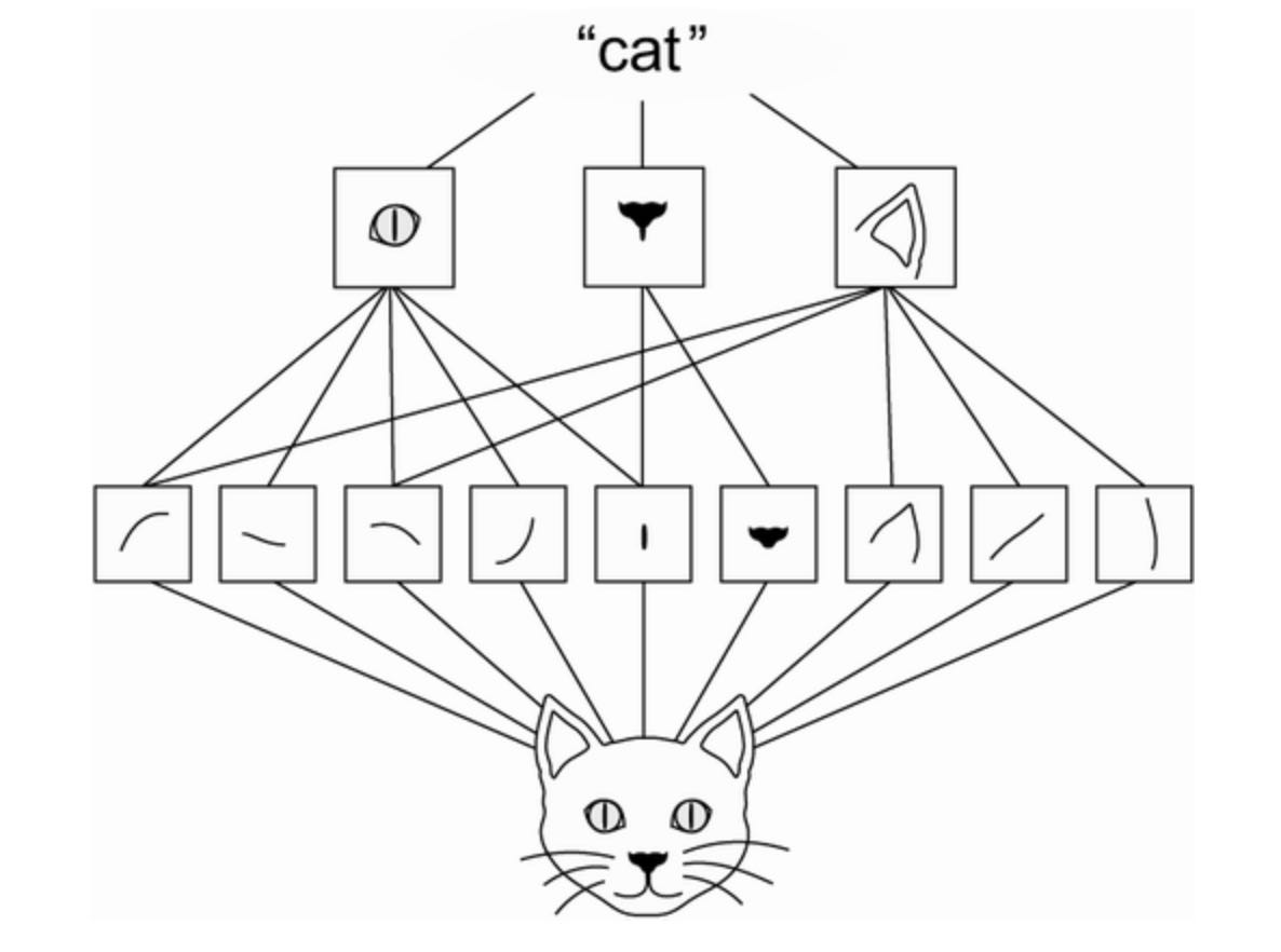
2. They can learn spatial hierarchies of patterns. A first convolution layer will learn small local patterns such as edges, a second convolution layer will learn larger patterns made of the features of the first layers, and so on. (see next figure). This allows convnets to efficiently learn increasingly complex and abstract visual concepts, because the visual world is fundamentally spatially hierarchical.

Convolutions operate over rank-3 tensors called feature maps, with two spatial axes (height and width) as well as a depth axis (also called the channel axis). For an RGB image, the dimension of the depth axis is 3, because the image has three color channels: red, green, and blue. For a black-and-white picture, like the MNIST digits, the depth is 1 (levels of gray). The convolution operation extracts patches from its input feature map and applies the same transformation to all of these patches, producing an output feature map. This output feature map is still a rank-3 tensor: it has a width and a height. Its depth can be arbitrary, because the output depth is a parameter of the layer, and the different channels in that depth axis no longer stand for specific colors as in RGB input; rather, they stand for filters. Filters encode specific aspects of the input data: at a high level, a single filter could encode the concept “presence of a face in the input”, for instance.

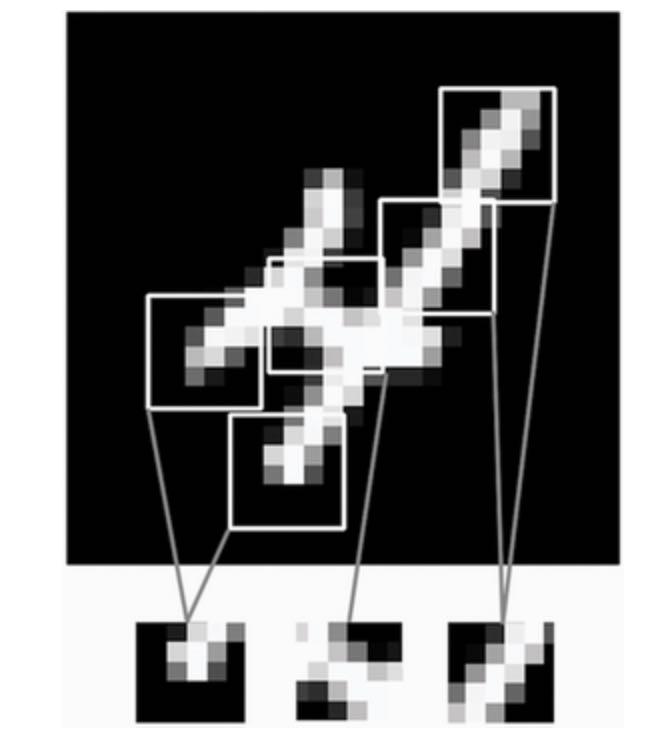
In the MNIST example, the first convolution layer takes a feature map of size (28, 28, 1) and outputs a feature map of size (26, 26, 32): it computes 32 filters over its input. Each of these 32 output channels contains a 26x26 grid of values, which is a response map of the filter over the input, indicating the response of that filter pattern at different locations in the input. (see next figure).

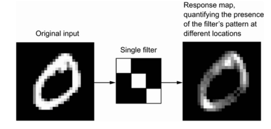
That is what the term feature map means: every dimension in the depth axis is a feature (or filter), and the rank-2 tensor output[:, :, n] is the 2D spatial map of the response of this filter over the input.

Convolutions are defined by two key parameters:

1. Size of the patches extracted from the inputs: These are typically 3x3 or 5x5. In the example, they were 3x3, which is a common choice.
2. Depth of the output feature map: The number of filters computed by the convolution. The example started with a depth of 32 and ended with a depth of 128.

In Keras Conv2D layers, these parameters are the first arguments passed to the layer: Conv2D(output_depth, (window_height, window_width)).

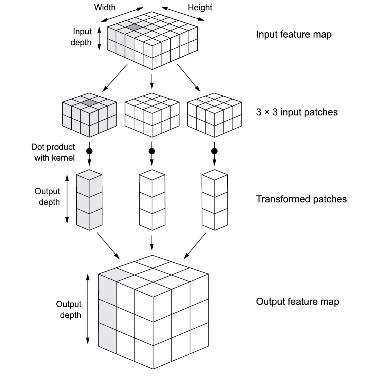
A convolution works by sliding these windows of size 3x3 or 5x5 over the 3D input feature map, stopping at every possible location, and extracting the 3D patch of surrounding features (shape (window_height, window_width, input_depth)). Each such 3D patch is then transformed into a 1D vector of shape (output_depth,) which is done via a tensor product with learned weight matrix, called the convolution kernel — the same kernel is reused across every patch. All of these vectors (one per patch) are then spatially reassembled into a 3D output map of shape (height, width, output_depth). Every spatial location in the output feature map corresponds to the same location in the input feature map (for example, the lower-right corner of the output contains information about the lower-right corner of the input). For instance, with 3x3 windows, the vector output[i, j, :] comes from the 3D patch input[i-1:i+1, j-1:j+1, :].

Note that the output width and height may differ from the input width and height for two reasons:

1. Border effects, which can be countered by padding the input feature map.
2. The use of strides.

Let’s take a deeper look at these notions.

UNDERSTANDING BORDER EFFECTS AND PADDING:

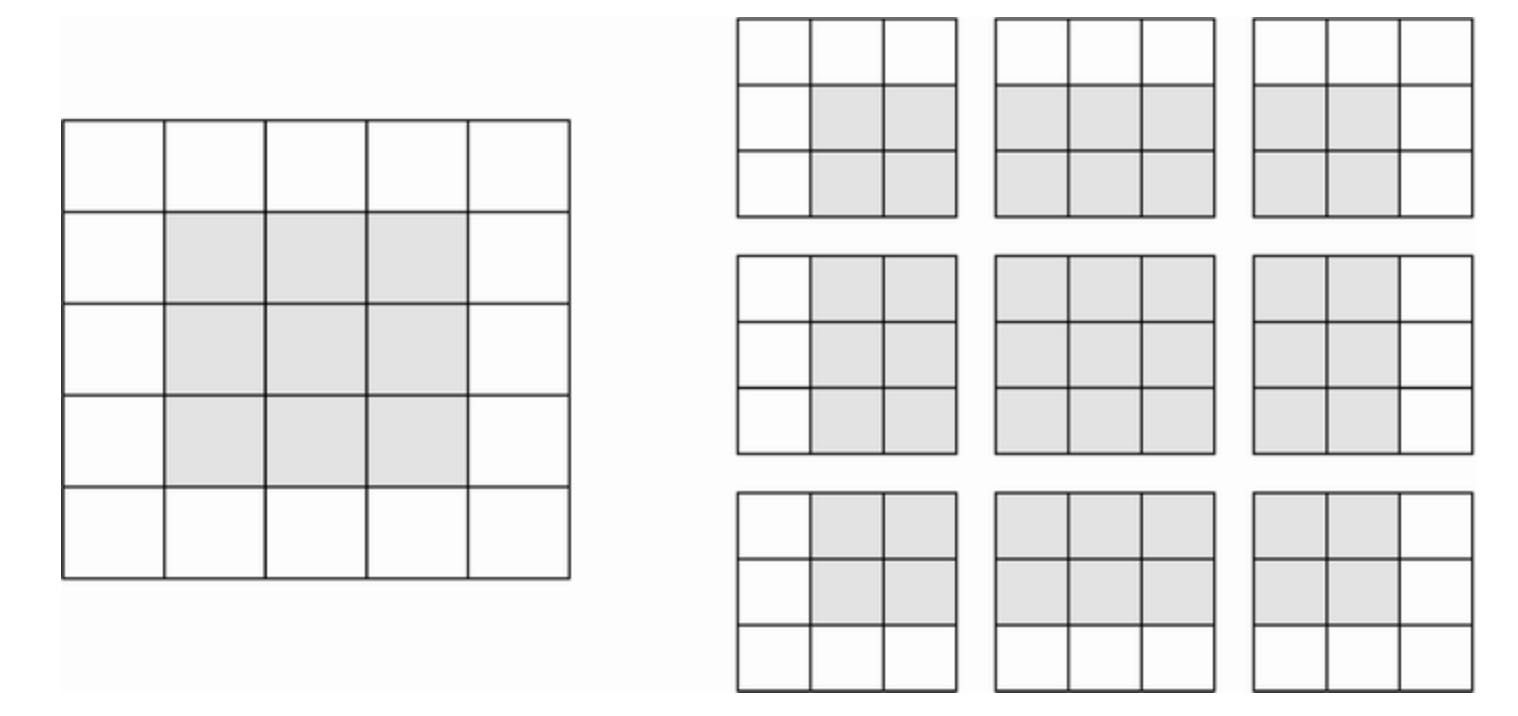
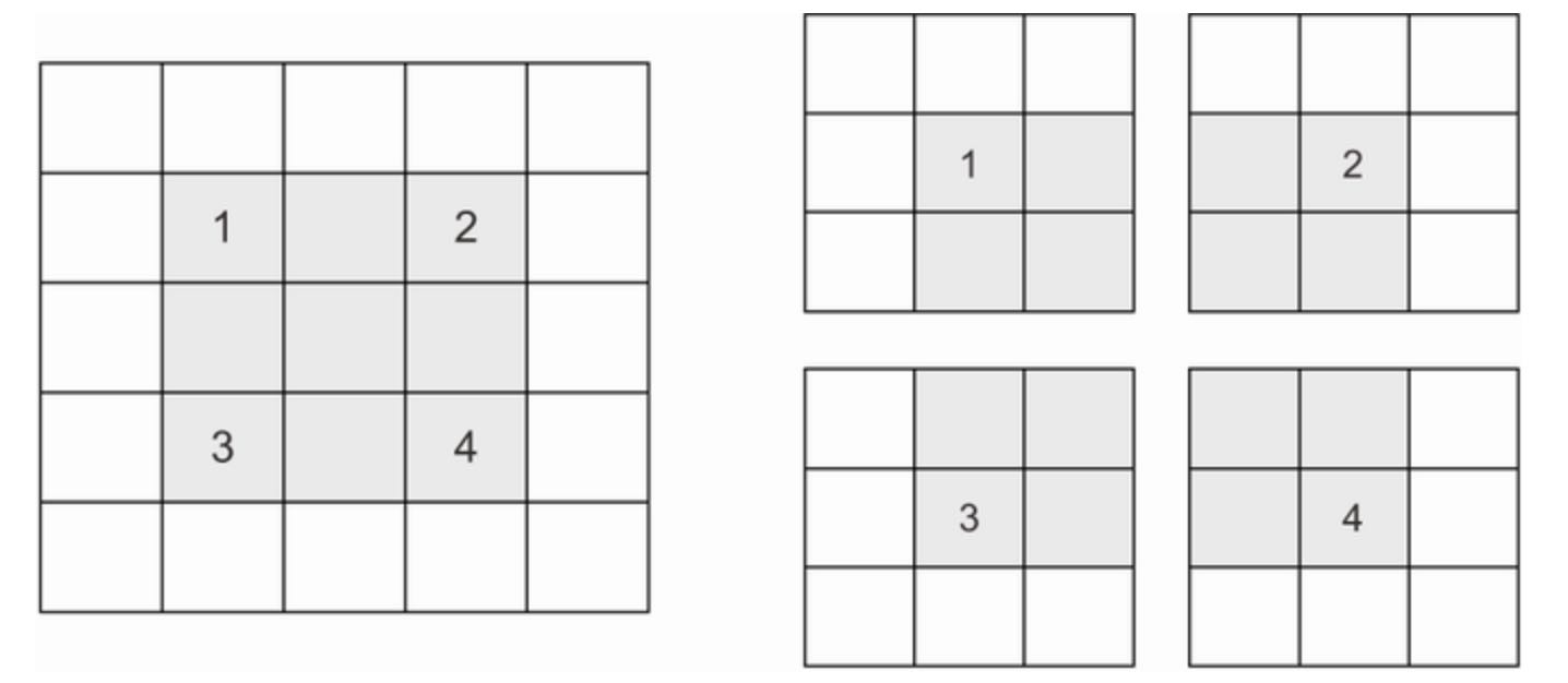
Consider a 5x5 feature map (25 tiles total). There are only 9 tiles around which you can center a 3x3 window, forming a 3x3 grid (see figure 8.5). Hence, the output feature map will be a 3x3. It shrinks a little: by exactly two tiles alongside each dimension, in this case. You can see this border effect in action in the earlier example: you start with 28x28 inputs, which become 26x26 after the first convolution layer.

If you want to get an output feature map with the same spatial dimensions as the input, you can use padding. Padding consists of adding an appropriate number of rows and columns on each side of the input feature map so as to make it possible to fit center convolution windows around every input tile. For a 3x3 window, you add one column on the right, one column on the left, one row at the top, and one row at the bottom. For a 5x5 window, you add two rows.

In Conv2D layers, padding is configurable via the padding argument, which takes two values: valid, which means no padding (only valid window locations will be used); and same, which means “pad in such a way as to have an output with the same width and height as the input”. The padding argument defaults to valid.

UNDERSTANDING CONVOLUTION STRIDES:

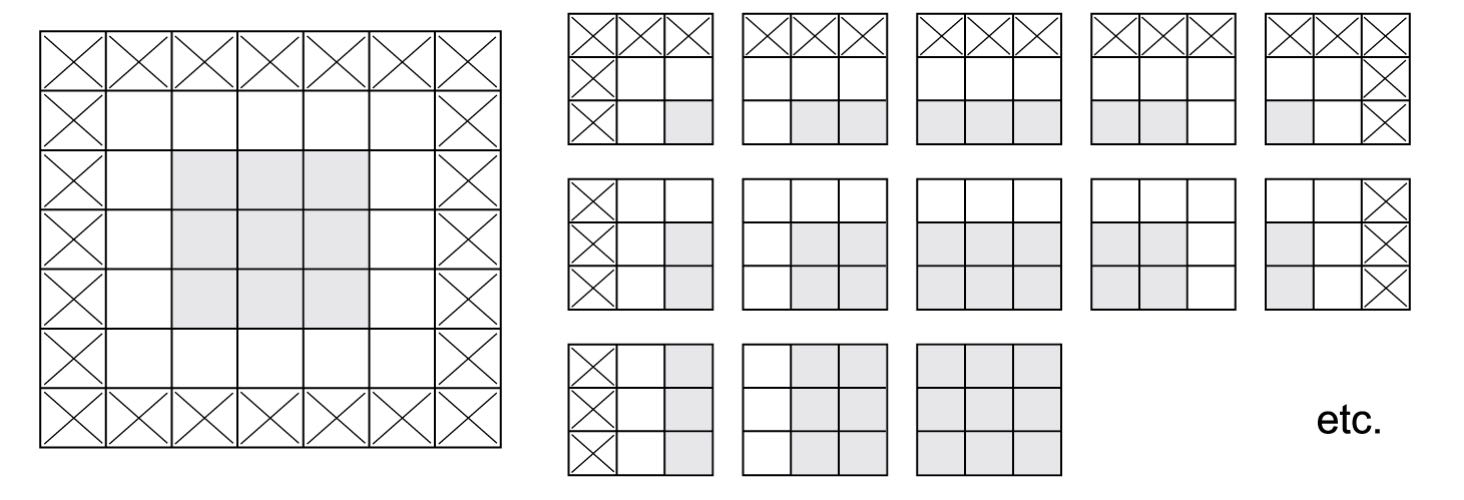
The other factor that can influence output size is the notion of strides. Our description of convolution so far has assumed that the center tiles of the convolution windows are all contiguous. But the distance between two successive windows is a parameter of the convolution, called its stride, which defaults to 1. It’s possible to have strided convolutions: convolutions with a stride higher than 1. In figure 8.7, you can see the patches extracted by a 3x3 convolution with stride 2 over a 5x5 input (without padding).

Using stride 2 means the width and height of the feature map are downsampled by a factor of 2 (in addition to any changes induced by border effects). Strided convolutions are rarely used in classification models, but they come in handy in some types of models, as you will see in next chapter.

In classification models, instead of strides, we tend to use the max-pooling operation to downsample feature maps, which you saw in action in our first convnet example. Let’s look at it in more depth.

8.1.2 The max-pooling operation

In the convnet example, you may have noticed that the size of the feature map is halved after every MaxPooling2D layer. For instance, before the first MaxPooling2D layers, the feature map is 26x26, but it becomes 13x13 after it. This is the role of max pooling: to aggressively downsample feature maps, much like strided convolutions.

Max pooling consists of extracting windows from the input feature maps and outputting the max value of each channel. It’s conceptually similar to convolution, except that instead of transforming local patches via a learned linear transformation (the convolution kernel), they are transformed via a hardcoded max tensor operation. A big difference from convolution is that max pooling is usually done with 2x2 windows and stride 2, in order to downsample the feature maps by a factor of 2. On the other hand, convolution is typically done with 3x3 windows and no stride (stride 1).

Why downsample feature maps this way? Why not remove the max-pooling layers and keep fairly large feature maps all the way up to the Dense layers? Let’s look at this option. Our model would then look like the following listing.

# Listing 8.5 An incorrectly structured convnet missing its max-pooling layers

inputs = keras.Input(shape=(28, 28, 1))
x = layers.Conv2D(filters=32, kernel_size=3, activation='relu')(inputs)
x = layers.Conv2D(filters=64, kernel_size=3, activation='relu')(x)
x = layers.Conv2D(filters=128, kernel_size=3, activation='relu')(x)
x = layers.Flatten()(x)
outputs = layers.Dense(10, activation='softmax')(x)
model_no_max_pool = keras.Model(inputs=inputs, outputs=outputs)

Let’s look at the model’s summary.

>>> model_no_max_pool.summary()
Model: "model_1"
_________________________________________________________________
Layer (type)                 Output Shape              Param #
=================================================================
input_2 (InputLayer)         [(None, 28, 28, 1)]       0
_________________________________________________________________
conv2d_3 (Conv2D)            (None, 26, 26, 32)        320
_________________________________________________________________
conv2d_4 (Conv2D)            (None, 24, 24, 64)        18496
_________________________________________________________________
conv2d_5 (Conv2D)            (None, 22, 22, 128)       73856
_________________________________________________________________
flatten_1 (Flatten)          (None, 61952)             0
_________________________________________________________________
dense_1 (Dense)              (None, 10)                619530
=================================================================
Total params: 712,202
Trainable params: 712,202
Non-trainable params: 0
_________________________________________________________________

What’s wrong with this setup? Two things:

• It isn’t conducive to learning spatial hierarchies of features. The 3x3 windows in the third layer will only contain information coming from 7x7 windows in the initial input. The high-level patterns learned by the convnet will still be very small with regard to the initial input, which may not be enough to learn to classify digits (try recognizing a digit by only looking at it through windows that are 7x7 pixels!). We need the features from the last convolution layer to contain information about the totality of the input.

• The final feature map has 22x22x128 = 61952 total coefficients per sample. This is huge. If you were to flatten it to stick a Dense layer of size 10 on top, that layer would have 619520 parameters. This is far too large for such a small model and would result in intense overfitting.

In short, the reason to use downsampling is to reduce the number of feature-map coefficients to process, as well as to induce spatial-filter hierarchies by making successive convolution layers look at increasingly large windows (in terms of the fraction of the original input they cover).

Note that max pooling isn’t the only way you can achieve such downsampling. As you already know, you can also use strides in the prior convolution layer. And you can use average pooling instead of max pooling, where each local input patch is transformed by taking the average value of each channel over the patch, rather than the max. But max pooling tends to work better than these alternative solutions. The reason is that features tend to encode the spatial presence of some pattern or concept over the different tiles of the feature map (hence, the term feature map), and it’s more informative to look at the maximal presence of different features than at their average presence. The most reasonable subsampling strategy is to first produce dense maps of features (via strided convolutions) or averaging input patches, which could cause you tomiss or dilute feature presence information.

At this point, you should understand the basics of convnets - feature maps, convolution, and max pooling - and you should know how to build a small convnet to solve a toy problem such as classifying MNIST digits. Now, let’s move on to more useful practical applications.

8.2 Training a convnet from scratch on a small dataset

Having to train an image-classification model using very little data is a common situation, which you will likely encounter in practice if you ever do computer vision in a professional context. A “few” samples can mean anywhere from a few hundred to a few tens of thousands of images. As a practical example, we will focus on classifying images as dogs or cats, in a dataset containing 5000 pictures of cats and dogs (2500 cats, 2500 dogs). We will use 2000 pictures for training, 1000 for validation, and 2000 for testing.

In this section we will review one basic strategy to tackle this problem: training a new model from scratch on what little data you have. We will start by naively training a small convnet on the 2000 training samples, without any regularization, to set a baseline for what can be achieved. This will get us to a classification accuracy of 70%. At that point, our main issue will be overfitting. Then we will introduce data augmentation, a powerful technique for mitigating overfitting in computer vision. By using data augmentation, we will improve the model to reach an accuracy of 80-85%.

In the next section, we will review two more essential techniques for applying deep learning to small datasets: feature extraction with a pretrained model (which will get us to an accuracy of 97.5%) and fine-tuning a pretrained model (which will get us to our final accuracy of 98.5%). Together, these three strategies - training a small model from scratch, doing feature extraction using a pretrained model, and fine-tuning a pretrained model - will constitute your future toolbox for tackling the problem of performing image classification with small datasets.

8.2.1 The relevance of deep learning for small-data problems

What qualifies as “enough samples” to train a model is relative - relative to the size and depth of the model you are trying to train, for starters. It isn’t possible to train a convnet to solve a complex problem with just a few tens of samples, but a few hundred can potentially suffice if the model is small and well regularized and if the task is simple. Because convnets learn local, translation-invariant features, they are highly data-efficient on perceptual problems. Training a convnet from scratch on a very small image dataset will yield reasonable results despite a relative lack of data, without the need for any custom feature engineering. You will see this in action in this section.

What’s more, deep learning models are by nature highly repurposable: you can take, say, an image-classification or speech-to-text model trained on a large-scale dataset and reuse it on a significantly different problem with only minor changes. Specifically, in the case of computer vision, many pre-trained models (usually trained on the ImageNet dataset) are now publicly available for download and can be used to bootstrap powerful vision models out of very little data. This is one of the greatest strengths of deep learning: feature reuse. You will explore this in the next section.

Let’s start by getting our hands on the data.

8.2.2 Downloading the data

The Dogs vs. Cats dataset that you will use isn’t packaged with Keras. It was made available by Kaggle as part of a computer vision competition in late 2013, back when convnets weren’t quite mainstream. You can download the original dataset from www.kaggle.com/c/dogs-vs-cats/data (you will need to create a Kaggle account if you don’t already have one - don’t worry, the process is painless). You can also use the Kaggle API to download the dataset in Colab (see the “Downloading a Kaggle dataset in Google Colaboratory” sidebar).

DOWNLOADING A KAGGLE DATASET IN GOOGLE COLABORATORY

Kaggle makes available an easy to use API to programmatically download Kaggle hosted datasets. You can use the Dogs vs Cats dataset to a Colab notebook, for instance. This API is available as the kaggle package, which is preinstalled on Colab. Downloading this dataset is as easy as running the following command in Colab shell:

!kaggle competitions download -c dogs-vs-cats

However, access to API is restricted to Kaggle users, so in order to run the preceding command, you first need to authenticate yourself. The kaggle package will look for your login credentials in a JSON file ~/.kaggle/kaggle.json. Let’s create this file. First, you need to create a Kaggle API key and download it to your local machine. Just navigate to the Kaggle website in a web browser, log in, and go to the My Account page. In your account settngs, you will find an API section. Clicking the Create New API Token button will generate a kaggle.json key file and will download it to your machine. Second, go to your Colab notebook, and upload the API’s key JSON file to your Colab session by running the following code in a notebook cell:

from google.colab import files
files.upload()

When you run this cell, you will see a Choose Files button appear. Click it and select the kaggle.json file you just downloaded. This uploads the file to the local Colab runtime. Finally, create a ~/.kaggle folder (mkdir ~/.kaggle) and copy the key file to it (cp kaggle.json ~/.kaggle/). As a security best practice, you should also make sure that the file is only readable by the current user, yourself (chmod 600).

!mkdir ~/.kaggle
!cp kaggle.json ~/.kaggle/
!chmod 600 ~/.kaggle/kaggle.json

You can now download the data we are about to use:

!kaggle competitions download -c dogs-vs-cats

The first time you try to download the data, you may get a “403 - Forbidden” error. This is because you need to accept the terms associated with the dataset before you downloa dit - you will have to go to www.kaggle.com/c/dogs-vs-cats/rules (while logged into your Kaggle account) and click I understand and accept button. You only need to do this once.

Once you’ve downloaded the data, uncompress (unzip) the archive (the -qq option means silently):

!unzip -qq dogs-vs-cats.zip

Finally, the training data is a compressed file named train.zip. Uncompress it:

!unzip -qq train.zip

The pictures in our dataset are medium-resolution color JPEGs. Here are a few samples:

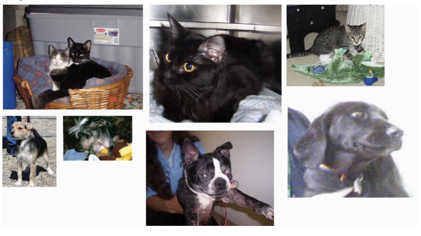
Unsurprisingly, the original dogs-vs-cats Kaggle competition, all the way back in 2013, was won by entrants who used convnets. The best entries achieved up to 95% accuracy. In our own example, we will get fairly close to this accuracy (in the next section), even though we will train our models on less than 10% of the data that was available to the competitors.

This dataset contains 25000 images of dogs and cats (12500 from each class) and is 543 MB large (compressed). After downloading and uncompressing the data, we will create a new dataset containing three subsets: a training set with 1000 samples of each class, a validation set with 500 samples of each class, and a test set with 1000 samples of each class. Why do this? Because many of the image datasets you’ll encounter in your career only contain a few thousand samples, not tens of thousands. Having more data available would make the problem easier, so it’s good practice to learn with a small dataset.

The subsampled dataset we will work with will have the following directory structure:

cats_vs_dogs_small/
    train/
        cat/  # Contains 1000 cat images
        dog/  # Contains 1000 dog images
    validation/
        cat/  # Contains 500 cat images
        dog/  # Contains 500 dog images
    test/
        cat/  # Contains 1000 cat images
        dog/  # Contains 1000 dog images

Let’s make it happen in a couple calls to shutil:

# Listing 8.6 Copying images to training, validation, and test directories

import os, shutil, pathlib

original_dir = pathlib.Path('train')  # Path to the directory where the original dataset was uncompressed
new_base_dir = pathlib.Path('cats_vs_dogs_small')  # Directory where we will store our smaller dataset

def make_subset(subset_name, start_index, end_index):  # Utility function to create subsets
    for category in ("cat", "dog"):
        dir = new_base_dir / subset_name / category
        os.makedirs(dir)
        fnames = [f"{category}.{i}.jpg" for i in range(start_index, end_index)]
        for fname in fnames:
            shutil.copyfile(src=original_dir / fname, dst=dir / fname)

make_subset("train", start_index=0, end_index=1000)  # Create training subset with 1000 samples of each category
make_subset("validation", start_index=1000, end_index=1500)  # Create validation subset with 500 samples of each category
make_subset("test", start_index=1500, end_index=2500)  # Create test subset with 1000 samples of each category

We now have 2000 training images, 1000 validation images, and 2000 test images. Each split contains the same number of samples from each class: this is a balanced binary-classification problem, which means classification accuracy will be an appropriate measure of success.

8.2.3 Building the model

We will reuse the same general structure you saw in the first example: the convnet will be a stack of alternated Conv2D (with relu activation) and MaxPooling2D layers.

But because we’re dealing with bigger images and a more complex problem, we will make our model larger, accordingly: it will have two more Conv2D and MaxPooling2D stages. This serves both to augment the capacity of the model and to further reduce the size of the feature maps so they aren’t overly large when we reach the Flatten layer. Here, because we start from inputs of size 180 pixels x 180 pixels (a somewhat arbitrary choice), we end up with feature maps of size 7x7 just before the Flatten layer.

Note: The depth of the feature maps progressively increases in the model (from 32 to 256), whereas the size of the feature maps decreases (from 180x180 to 7x7). This is a pattern you will see in almost all convnets.

Because we are looking at a binary classification problem, we will end the model with a single unit (a Dense layer of size 1) and a sigmoid activation. This unit will encode the probability that the model is looking at one class or the other.

One last small difference: we will start th model with a Rescaling layer, which will rescale image inputs (whose values are originally in the [0, 255] range) to the [0, 1] range.

# Listing 8.7 Instantiating a small convnet for dogs vs. cats classification

from tensorflow import keras
from tensorflow.keras import layers

inputs = keras.Input(shape=(180, 180, 3))
x = layers.Rescaling(1.0 / 255)(inputs)
x = layers.Conv2D(filters=32, kernel_size=3, activation='relu')(x)
x = layers.MaxPooling2D(pool_size=2)(x)
x = layers.Conv2D(filters=64, kernel_size=3, activation='relu')(x)
x = layers.MaxPooling2D(pool_size=2)(x)
x = layers.Conv2D(filters=128, kernel_size=3, activation='relu')(x)
x = layers.MaxPooling2D(pool_size=2)(x)
x = layers.Conv2D(filters=256, kernel_size=3, activation='relu')(x)
x = layers.MaxPooling2D(pool_size=2)(x)
x = layers.Conv2D(filters=256, kernel_size=3, activation='relu')(x)
x = layers.MaxPooling2D(pool_size=2)(x)
x = layers.Flatten()(x)
outputs = layers.Dense(1, activation='sigmoid')(x)
model = keras.Model(inputs=inputs, outputs=outputs)

Let’s look at how the dimensions of the feature maps change with every successive layer:

>>> model.summary()
Model: "model_2"
_________________________________________________________________
Layer (type)                 Output Shape              Param #
=================================================================
input_3 (InputLayer)         [(None, 180, 180, 3)]     0
_________________________________________________________________
rescaling (Rescaling)        (None, 180, 180, 3)       0
_________________________________________________________________
conv2d_6 (Conv2D)            (None, 178, 178, 32)      896
_________________________________________________________________
max_pooling2d_2 (MaxPooling2 (None, 89, 89, 32)        0
_________________________________________________________________
conv2d_7 (Conv2D)            (None, 87, 87, 64)        18496
_________________________________________________________________
max_pooling2d_3 (MaxPooling2 (None, 43, 43, 64)        0
_________________________________________________________________
conv2d_8 (Conv2D)            (None, 41, 41, 128)       73856
_________________________________________________________________
max_pooling2d_4 (MaxPooling2 (None, 20, 20, 128)       0
_________________________________________________________________
conv2d_9 (Conv2D)            (None, 18, 18, 256)       295168
_________________________________________________________________
max_pooling2d_5 (MaxPooling2 (None, 9, 9, 256)         0
_________________________________________________________________
conv2d_10 (Conv2D)           (None, 7, 7, 256)         590080
_________________________________________________________________
flatten_2 (Flatten)          (None, 12544)             0
_________________________________________________________________
dense_2 (Dense)              (None, 1)                 12545
=================================================================
Total params: 991,041
Trainable params: 991,041
Non-trainable params: 0
_________________________________________________________________

For the compilation step, we will go with the RMSprop optimizer, as usual. Because we ended the model with a single sigmoid unit, we will use binary_crossentropy as the loss (as a reminder, check out table 6.1 for a cheat sheet on which loss function to use in various situations).

# Listing 8.8 Configuring the model for training

model.compile(optimizer='rmsprop',
              loss='binary_crossentropy',
              metrics=['accuracy'])

8.2.4 Data preprocessing

As you know by now, data should be formatted into appropriately preprocessed floating-point tensors before being fed into the model. Currently, the data sits on a drive as JPEG files, so the steps for getting it into the model are roughly as follows:

1. Read the picture files.
2. Decode the JPEG content to RGB grids of pixels.
3. Convert these into floating-point tensors.
4. Resize them to a shared size (we’ll use 180x180).
5. Pack them into batches (we’ll use batches of 32 images).

It may seem a bit daunting, but fortunately Keras has utilities to take care of these steps automatically. In particular, Keras features the utility function image_dataset_from_directory, which lets you quickly set up a data pipeline that can automatically turn image files on disk into batches of preprocessed tensors. This is what we will use here.

Calling image_dataset_from_directory will first list the subdirectories of directory and assume each one contains images from one of our classes. It will then index the image files in each subdirectory. Finally, it will create and return a tf.data.Dataset object configured to read these files, shuffle them, decode them to tensors, resize them to a shared size, and pack them into batches.

# Listing 8.9 Using image_dataset_from_directory to read images

from tensorflow.keras.utils import image_dataset_from_directory

train_dataset = image_dataset_from_directory(
    directory=new_base_dir / "train",
    image_size=(180, 180),
    batch_size=32)
validation_dataset = image_dataset_from_directory(
    directory=new_base_dir / "validation",
    image_size=(180, 180),
    batch_size=32)
test_dataset = image_dataset_from_directory(
    directory=new_base_dir / "test",
    image_size=(180, 180),
    batch_size=32)

SIDENOTE BEGINS:

Understanding TensorFlow Dataset objects:

TensorFlow makes available tf.data API to create efficient input pipelines for machine learning models. Its core class is tf.data.Dataset.

A Dataset object is an iterator: you can use it in a for loop. It will typically return batches of input data and labels. You can pass a Dataset object directly to the fit() method of a Keras model.

The Dataset class handles many key features that would otherwise be cumbersome to implement yourself - in particular, asynchronous data prefetching (preprocessing the next batch of data while the previous one is being handled by the model, which keeps execution flowing without interruptions).

The Dataset class also exposes a functional-style API for modifying datasets. Here’s a quick example: let’s create a Dataset instance from NumPy array of random numbers. We will consider 1000 samples, where each sample is a vector of size 16:

import numpy as np
import tensorflow as tf

random_numbers = np.random.normal(size=(1000, 16))
dataset = tf.data.Dataset.from_tensor_slices(random_numbers)  # The from_tensor_slices() method can be used to create a Dataset from a NumPy array, or a tuple or a dict of NumPy arrays.

At first, our dataset just yields single samples:

>>> for i, element in enumerate(dataset):
>>>     print(element.shape)
>>>     if i >= 2:
>>>         break
(16,)
(16,)
(16,)

We can use the .batch() method to batch the data:

>>> batched_dataset = dataset.batch(32)
>>> for i, element in enumerate(batched_dataset):
>>>     print(element.shape)
>>>     if i >= 2:
>>>         break
(32, 16)
(32, 16)
(32, 16)

More broadly, we have access to a range of useful dataset methods, such as:

• .shuffle(buffer_size): Shuffles elements within a buffer.
• .prefetch(buffer_size): Prefetches a buffer of elements in GPU memory to achieve better device utilization.
• .map(callable): Applies an arbitrary transformation to each element of the dataset (the function callable, which expects to take as input a single element yielded by the dataset).

The .map() method, in particular, is one that you will use often. Here’s an example. We’ll use it to reshape the elements in our toy dataset from shape (16,) to shape (4, 4):

>>> reshaped_dataset = dataset.map(lambda x: tf.reshape(x, shape=(4, 4)))
>>> for i, element in enumerate(reshaped_dataset):
>>>     print(element.shape)
>>>     if i >= 2:
>>>         break
(4, 4)
(4, 4)
(4, 4)

You are about to see more map() action in this chapter.

SIDENOTE ENDED.

Back to the dogs vs. cats example:

Let’s look at the output of one of these Dataset objects: it yields batches of 180 x 180 RGB images (shape (32, 180, 180, 3)) and integer labels (shape (32,)). There are 32 samples in each batch (the batch size we used when calling image_dataset_from_directory).

# Listing 8.10 Displaying the shapes of the data and labels yielded by the Dataset

>>> for data_batch, labels_batch in train_dataset:
>>>     print(f"data batch shape: {data_batch.shape}")
>>>     print(f"labels batch shape: {labels_batch.shape}")
>>>     break
data batch shape: (32, 180, 180, 3)
labels batch shape: (32,)

Let’s fit the model on our dataset. We’ll use the validation_data argument in fit() to monitor validation metrics on a separate Dataset object.

Note that we’ll also use a ModelCheckpoint callback to save the model after each epoch. We’ll configure it with the path specifying where to save the file, as well as the arguments save_best_only=True and monitor='val_loss': they tell the callback to only save a new file (overwriting any previous one) when the current value of the val_loss metric is lower than at any previous time during training. This guarantees that your saved file will always contain the state of the model corresponding to its best performing training epoch, in terms of its performance on the validation data. As a result, we won’t have to retrain a new model for a lower number of epochs if we start overfitting: we can just reload our saved file.

# Listing 8.11 Fitting the model using a Dataset
callbacks = [
    keras.callbacks.ModelCheckpoint(
        filepath="convnet_from_scratch.keras",
        save_best_only=True,
        monitor="val_loss",
    )
]

history = model.fit(
    train_dataset,
    epochs=30,
    validation_data=validation_dataset,
    callbacks=callbacks)

Let’s plot the loss and accuracy of the model over the training and validation data during training:

# Listing 8.12 Displaying curves of loss and accuracy during training

import matplotlib.pyplot as plt
accuracy = history.history['accuracy']
val_accuracy = history.history['val_accuracy']
loss = history.history['loss']
val_loss = history.history['val_loss']
epochs = range(1, len(accuracy) + 1)
plt.plot(epochs, accuracy, 'bo', label='Training accuracy')
plt.plot(epochs, val_accuracy, 'b', label='Validation accuracy')
plt.title('Training and validation accuracy')
plt.legend()
plt.figure()
plt.plot(epochs, loss, 'bo', label='Training loss')
plt.plot(epochs, val_loss, 'b', label='Validation loss')
plt.title('Training and validation loss')
plt.legend()
plt.show()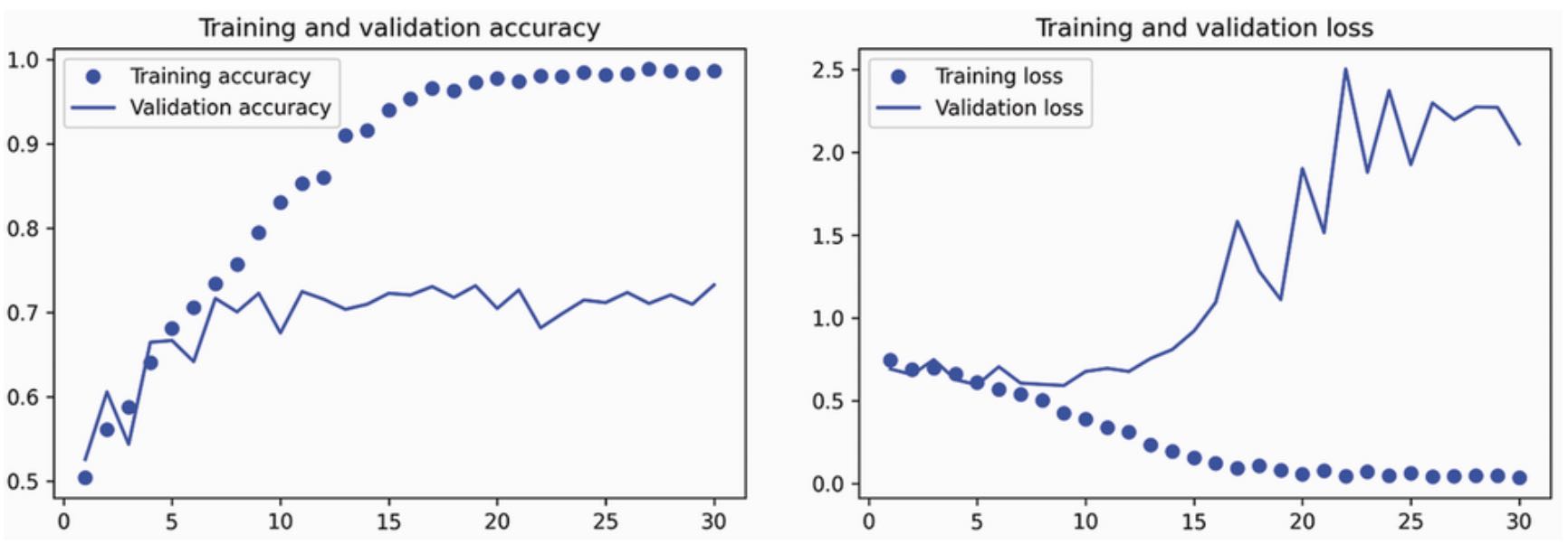

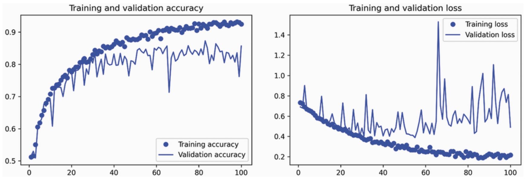
These plots are characteristic of overfitting. The training accuracy increases linearly over time, until it reaches nearly 100%, whereas the validation accuracy peaks at 75%. The validation loss reaches its minimum after only ten epochs and then stalls, whereas the training loss keeps decreasing linearly as training proceeds.

Let’s check the test accuracy. We’ll reload the model from its saved file to evaluate it as it was before it started overfitting.

# Listing 8.13 Evaluating the model on the test set

test_model = keras.models.load_model("convnet_from_scratch.keras")
test_loss, test_acc = test_model.evaluate(test_dataset)
print(f"Test accuracy: {test_acc:.3f}")

We get a test accuracy of 69.5%. (Due to randomness of neural network initializations, you may get numbers within one percentage point of that.)

Because we have relatively few training samples (2000), overfitting will be our number one concern. You already know about a number of techniques that can help mitigate overfitting, such as dropout and weight decay (L2 regularization). We’re now going to work with a new one, specific to computer vision, and used almost universally when processing images with deep learning models: data augmentation.

8.2.5 Using data augmentation

Overfitting is caused by having too few samples to learn from, rendering you unable to train a model that can generalize to new data. Given infinite data, your model would be exposed to every possible aspect of data distribution at hand: you would never overfit. Data augmentation takes the approach of generating more training data from existing training samples by augmenting the samples via a number of random transformations that yield believable-looking images. The goal is that at training time, your model will never see the exact same picture twice. This helps expose the model to more aspects of the data and generalize better.

In Keras, this can be done by adding a number of data augmentation layers at the start of your model. Let’s get started with an example: the following Sequential model chains several random image transformations. In our model, we’d include it right before the Rescaling layer:

# Listing 8.14 Define a data augmentation stage to add to an Image model

data_augmentation = keras.Sequential(
    [
        layers.RandomFlip("horizontal"),
        layers.RandomRotation(0.1),
        layers.RandomZoom(0.2),
        # layers.RandomContrast(0.2),
    ]
)

These are just a few of the layers available (for more, see the Keras documentation). Let’s quickly go over this code:

• RandomFlip("horizontal") : Applies horizontal flipping to a random 50% of the images that go through it.
• RandomRotation(0.1) : Rotates the input images by a random value in the range [-10%, +10%] (these are fractions of a full circle - in degrees, the range would be [-36°, +36°]).
• RandomZoom(0.2) : Zooms in or out of the image by a random factor in the range [-20%, +20%].

Let’s look at the augmented images(see figure 8.10):

# Listing 8.15 Displaying some randomly augmented training images

import matplotlib.pyplot as plt
plt.figure(figsize=(10, 10))

# We can use take(N) to only sample N batches from the dataset. This is equivalent to inserting a break in the loop after the Nth batch.
for images, _ in train_dataset.take(1):
    for i in range(9):
        # Apply the augmentation stage to the batch of images
        augmented_images = data_augmentation(images)
        ax = plt.subplot(3, 3, i + 1)
        plt.imshow(augmented_images[0].numpy().astype("uint8"))  # Display the first image in the output batch. For each of the nine iterations, this is a different augmentation of the same image.
        plt.axis("off")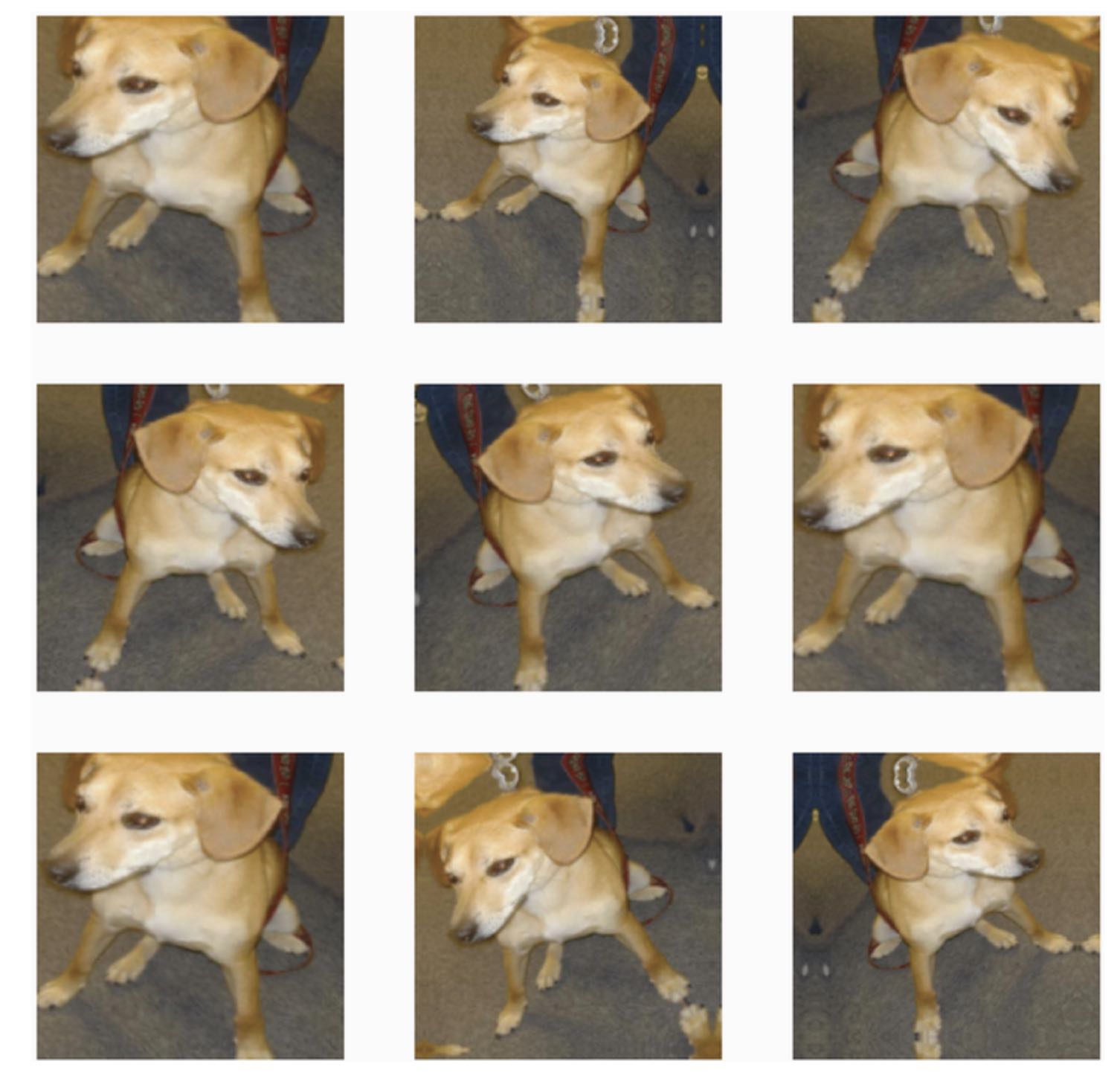

If we train a new model using this data-augmentation configuration, the model will never see the same input twice. But the inputs it sees are still heavily intercorrelated because they come from a small number of original images - we can’t produce new information, we can only remix existing information. As such, this may not be enough to completely get rid of overfitting. To further fight overfitting, we will also add a Dropout layer right before the densely connected classifier.

One last thing you should know about random image augmentation layers: just like Dropout, they’re inactive during inference (when we call predict() or evaluate()). During evaluation, out model will behave just the same as when it did not include data augmentation and dropout.

# Listing 8.16 Defining a new convnet that includes image augmentation and dropout

inputs = keras.Input(shape=(180, 180, 3))
x = data_augmentation(inputs)
x = layers.Rescaling(1.0 / 255)(x)
x = layers.Conv2D(filters=32, kernel_size=3, activation='relu')(x)
x = layers.MaxPooling2D(pool_size=2)(x)
x = layers.Conv2D(filters=64, kernel_size=3, activation='relu')(x)
x = layers.MaxPooling2D(pool_size=2)(x)
x = layers.Conv2D(filters=128, kernel_size=3, activation='relu')(x)
x = layers.MaxPooling2D(pool_size=2)(x)
x = layers.Conv2D(filters=256, kernel_size=3, activation='relu')(x)
x = layers.MaxPooling2D(pool_size=2)(x)
x = layers.Conv2D(filters=256, kernel_size=3, activation='relu')(x)
x = layers.MaxPooling2D(pool_size=2)(x)
x = layers.Flatten()(x)
x = layers.Dropout(0.5)(x)  # Add a dropout layer
outputs = layers.Dense(1, activation='sigmoid')(x)
model = keras.Model(inputs=inputs, outputs=outputs)

model.compile(optimizer='rmsprop',
              loss='binary_crossentropy',
              metrics=['accuracy'])

Let’s train the model using data augmentation and dropout. Because we expect overfitting to occur much later during training, we will train for three times as many epochs - one hundred.

# Listing 8.17 Training the regularized convnet

callbacks = [
    keras.callbacks.ModelCheckpoint(
        filepath="convnet_with_data_augmentation.keras",
        save_best_only=True,
        monitor="val_loss",
    )
]

history = model.fit(
    train_dataset,
    epochs=100,
    validation_data=validation_dataset,
    callbacks=callbacks)

Let’s plot the results again: see figure 8.11. Thanks to data augmentation and dropout, we start overfitting much later, around epochs 60-70(compared to epoch 10 for the original model). The validation accuracy ends up consistently in the 80-85% range - a big improvement over our first cry.

Let’s check the test accuracy:

# Listing 8.18 Evaluating the model on the test set

test_model = keras.models.load_model("convnet_with_data_augmentation.keras")
test_loss, test_acc = test_model.evaluate(test_dataset)
print(f"Test accuracy: {test_acc:.3f}")

We get a test accuracy of 83.5%. It’s starting to look good! If you are using Colab, make sure you download the saved file (convnet_with_data_augmentation.keras) as we will use it for some experiments in the next chapter.

By further tuning the model’s configuration (such as the number of filters per convolution layer, or the number of layers in the model), , we might be able to get an even better accuracy, likely upto 90%. But it would prove difficult to go any higher just by training our own convnet from scratch, because we have so little data to work with. As a next step to improve our accuracy on this problem, we’ll have to use a pretrained model, which is the focus of next two sections.

8.3 Leveraging a pretrained model

A common and highly effective approach to deep learning on small image datasets is to use a pretrained model. A pretrained model is a model that was previously trained on a large dataset, typically on a large-scale image-classification task. If this original dataset is large enough and general enough, then the spatial hierarchy of features learned by the pretrained model can effectively act as a generic model of our visual world, and hence its features can prove useful for many different computer vision problems, even though these new problems might involve completely different classes than those of the original task. For instance, you might train a model on ImageNet (where classes are mostly animals and everyday objects) and then repurpose this trained model for something as remote as identifying furniture items in images. Such portability of learned features across different problems is a key advantage of deep learning compared to many older, shallow-learning approaches, and it makes deep learning very effective for small-data problems.

In this case, let’s consider a large convnet trained on the ImageNet dataset (1.4 million labeled images and 1000 different classes). ImageNet contains many animal classes, including different species of cats and dogs, and you can thus expect it to perform well on the dogs vs. cats classification problem.

We will use the VGG16 architecture, developed by Karen Simonyan and Andrew Zisserman in 2014. Although it’s an older model, far from the current state of the art and somewhat heavier than many other recent models, we chose it because its architecture is similar to what you are already familiar with and easy to understand without introducing any new concepts. This may be your first encounter with one of these cutesy model name - VGG, ResNet, Inception, Inception-ResNet, Xception, and so on. You will get used to them because they will come up frequently if you keep doing deep learning for computer vision.

There are two ways to use a pretrained model: feature extraction and fine-tuning. We will cover both. Let’s start with feature extraction.

8.3.1 Feature extraction

Feature extraction consists of using the representations learned by a previously trained model to extract interesting features from new samples. These features are then run through a new classifier, which is trained from scratch.

As we saw earlier, convnets used for image classification comprise two parts: they start with a series of pooling and convolution layers, and they end with a densely connected classifier. The first part is called the convolutional base of the model. In the case of convnets, feature extraction consists of taking the convolutional base of a previously trained network, running the new data through it, and training a new classifier on top of the output. (see figure 8.12).

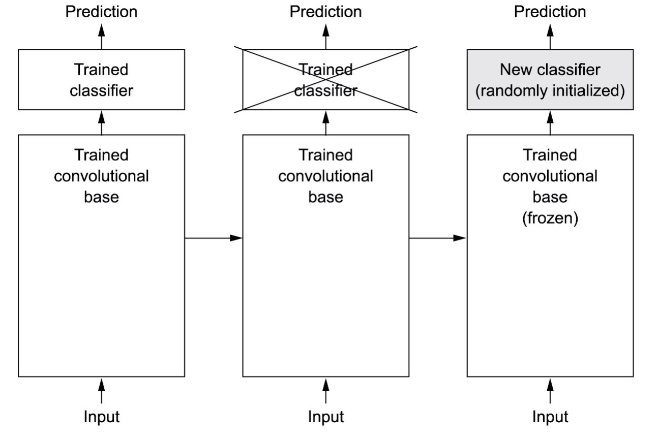
Why only resuse the convolutional base? Could we reuse the densely connected classifier as well? In general, it should be avoided. The reason is that the representations learned by the convolutional base are likely to be more generic and therefore more reusable: the feature maps of a convnet are presence maps of generic concepts over a picture, which are likely to be useful regardless of the computer vision problem at hand. On the other hand, the representations learned by the classifier will necessarily be specific to the set of classes on which the model was trained - they will only contain information about the presence probability of this or that class in the entire picture. Additionally, representations found in densely connected layers no longer contain any information about where objects are located in the input image: these layers get rid of the notion of space, whereas the object location is still described by convolutional feature maps. For problems where object location matters, densely connected features would be largely useless.

Note that the level of generality (and therefore reusability) of the representations extracted by specific convolution layers depends on the depth of the layer in the model. Layers that come earlier in the model extract local, highly generic feature maps (such as visual edges, colors, and textures), whereas layers that are higher up extract more abstract concepts (such as “cat ear” or “dog eye”). So if your new dataset differs a lot from the dataset on which the original model was trained, you may be better off using only the first few layers of the model to do feature extraction, rather than using the entire convolutional base.

In this case, because the ImageNet class set contains multiple dog and cat classes, it’s likely to be beneficial to reuse the information contained in the densely connected layers of the original model. But we’ll choose not to, in order to cover the more general case where the class set of the new problem doesn’t overlap with the class set of the original model. Let’s put this in practice by using the convolutional base of the VGG16 network, trained on ImageNet, to extract interesting features from cats and dogs images, and then train a dogs vs. cats classifier on top of these features.

The VGG16 model, among others, comes prepackaged with Keras. You can import it from the keras.applications module. Many other image-classification models(all pretrained on the ImageNet dataset) are available as part of keras.applications:

• Xception
• ResNet
• MobileNet
• EfficientNet
• DenseNet
• etc.

Let’s instantiate the VGG16 model:

# Listing 8.19 Instantiating the VGG16 convolutional base

conv_base = keras.applications.vgg16.VGG16(
    weights='imagenet',
    include_top=False,  # We won't use the densely connected classifier
    input_shape=(180, 180, 3))

We pass three arguments to the constructor:

• weights specifies the weight checkpoint from which to initialize the model.
• include_top refers to including (or not) the densely connected classifier on top of the network. By default, this densely connected classifier corresponds to the 1000 classes from ImageNet. Because we intend to use our own densely connected classifier (with only two classes: cat and dog), we don’t need to include it.
• input_shape is the shape of the image tensors that we will feed to the network. This argument is purely optional: if we don’t pass it, the network will be able to process inputs of any size. Here we pass it so that we can visualize (in the following summary) how the size of the feature maps shrinks with each new convolutional and pooling layer.

Here’s the detail of the architecture of the VGG16 convolutional base. It’s similar to the simple convnets you are already familiar with:

>>> conv_base.summary()
Model: "vgg16"
_________________________________________________________________
Layer (type)                 Output Shape              Param #
=================================================================
input_19 (InputLayer)        [(None, 180, 180, 3)]     0
_________________________________________________________________
block1_conv1 (Conv2D)        (None, 180, 180, 64)      1792
_________________________________________________________________
block1_conv2 (Conv2D)        (None, 180, 180, 64)      36928
_________________________________________________________________
block1_pool (MaxPooling2D)   (None, 90, 90, 64)        0
_________________________________________________________________
block2_conv1 (Conv2D)        (None, 90, 90, 128)       73856
_________________________________________________________________
block2_conv2 (Conv2D)        (None, 90, 90, 128)       147584
_________________________________________________________________
block2_pool (MaxPooling2D)   (None, 45, 45, 128)       0
_________________________________________________________________
block3_conv1 (Conv2D)        (None, 45, 45, 256)       295168
_________________________________________________________________
block3_conv2 (Conv2D)        (None, 45, 45, 256)       590080
_________________________________________________________________
block3_conv3 (Conv2D)        (None, 45, 45, 256)       590080
_________________________________________________________________
block3_pool (MaxPooling2D)   (None, 22, 22, 256)       0
_________________________________________________________________
block4_conv1 (Conv2D)        (None, 22, 22, 512)       1180160
_________________________________________________________________
block4_conv2 (Conv2D)        (None, 22, 22, 512)       2359808
_________________________________________________________________
block4_conv3 (Conv2D)        (None, 22, 22, 512)       2359808
_________________________________________________________________
block4_pool (MaxPooling2D)   (None, 11, 11, 512)       0
_________________________________________________________________
block5_conv1 (Conv2D)        (None, 11, 11, 512)       2359808
_________________________________________________________________
block5_conv2 (Conv2D)        (None, 11, 11, 512)       2359808
_________________________________________________________________
block5_conv3 (Conv2D)        (None, 11, 11, 512)       2359808
_________________________________________________________________
block5_pool (MaxPooling2D)   (None, 5, 5, 512)         0
=================================================================
Total params: 14,714,688
Trainable params: 14,714,688
Non-trainable params: 0
_________________________________________________________________

The final feature map has shape (5, 5, 512). That’s the feature on top of which we will stick a densely connected classifier.

At this point, there are two ways we could proceed:

• Run the convolutional base over our dataset, record its output to a Numpy array on disk, and then use this data as input to a standalone, densely connected classifier similar to those you saw in chapter 4. This solution is fast and cheap to run, because it only requires running the convolutional base once for every input image, and the convolutional base is by far the most expensive part of the pipeline. But for the same reason, this technique won’t allow us to use data augmentation.

• Extend the model we have (conv_base) by adding Dense layers on top, and run the whole thing end to end on the input data. This will allow us to use data augmentation, because every input image will go through the convolutional base every time it’s seen by the model. But for the same reason, this technique is far more expensive than the first.

We will cover both techniques. Let’s walk through the code required to set up the first one: recording the output of conv_base on our data and using these outputs as inputs to a new model.

FAST FEATURE EXTRACTION WITHOUT DATA AUGMENTATION:

We’ll start by extracting features as NumPy arrays be calling the predict() method of the conv_base model on our training, validation, and testing datasets.

Let’s iterate over our datasets to extract the VGG16 features.

# Listing 8.20 Extracting the VGG16 features and corresponding labels

import numpy as np

def get_features_and_labels(dataset):
    all_features = []
    all_labels = []
    for images, labels in dataset:
        preprocessed_images = keras.applications.vgg16.preprocess_input(images)
        features = conv_base.predict(preprocessed_images)
        all_features.append(features)
        all_labels.append(labels)
    return np.concatenate(all_features), np.concatenate(all_labels)

train_features, train_labels = get_features_and_labels(train_dataset)
val_features, val_labels = get_features_and_labels(validation_dataset)
test_features, test_labels = get_features_and_labels(test_dataset)

Importantly, predict() only expects images, not labels, but our current dataset yields batches that contain both images and their labels. Moreover, the VGG16 model expects inputs that are preprocessed with the function keras.applications.vgg16.preprocess_input, which scales pixel values to an appropriate range.

The extracted features are currently of shape (samples, 5, 5, 512):

>>> train_features.shape
(2000, 5, 5, 512)

At this point, we can define our densely connected classifier (note the use of dropout for regularization) and train it on the data and labels that we just recorded:

# Listing 8.21 Defining and training the densely connected classifier

inputs = keras.Input(shape=(5, 5, 512))
x = layers.Flatten()(inputs)  # Note the use of the Flatten layer to flatten layer before passing the features to the Dense layer
x = layers.Dense(256)(x)
x = layers.Dropout(0.5)(x)
outputs = layers.Dense(1, activation='sigmoid')(x)
model = keras.Model(inputs=inputs, outputs=outputs)

model.compile(optimizer='rmsprop',
              loss='binary_crossentropy',
              metrics=['accuracy'])


callbacks = [
    keras.callbacks.ModelCheckpoint(
        filepath="feature_extraction.keras",
        save_best_only=True,
        monitor="val_loss",
    )
]

history = model.fit(
    train_features, train_labels,
    epochs=20,
    validation_data=(val_features, val_labels),
    callbacks=callbacks)

Training is very fast because we only have to deal with two Dense layers - an epoch takes less than one second on a CPU.

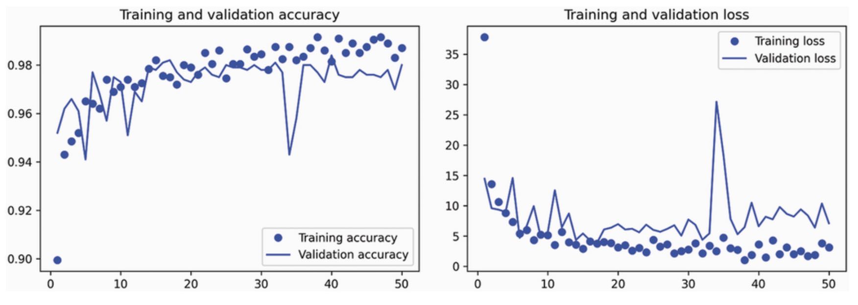
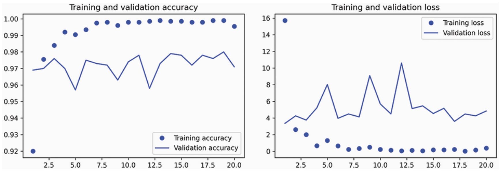
Let’s look at the loss and accuracy curves during training (see figure 8.13):

# Listing 8.22 Plotting the results

import matplotlib.pyplot as plt

acc = history.history['accuracy']
val_acc = history.history['val_accuracy']
loss = history.history['loss']
val_loss = history.history['val_loss']
epochs = range(1, len(acc) + 1)
plt.plot(epochs, acc, 'bo', label='Training accuracy')
plt.plot(epochs, val_acc, 'b', label='Validation accuracy')
plt.title('Training and validation accuracy')
plt.legend()
plt.figure()
plt.plot(epochs, loss, 'bo', label='Training loss')
plt.plot(epochs, val_loss, 'b', label='Validation loss')
plt.title('Training and validation loss')
plt.legend()
plt.show()

We reach a validation accuracy of about 97% - much better than we achieved in the previous section, with the small model trained from scratch. This is a bit of an unfair comparison, because the ImageNet

SUMMARY

Previous Chapter Next Chapter